A new session from GTC shares how to use synthetic data and Fleet Command to deploy highly accurate and scalable models.
The retail supply chain is complex and includes everything from creating a product, distributing it, putting it on shelves in stores, to getting it into customer hands. Retailers and Consumer Packaged Goods (CPG) companies must look at the entire supply chain for critical gaps and problems that can be solved with technology and automation. Computer vision has been implemented by many of these companies for years, with cameras distributed in their stores, warehouses, and on assembly lines. This is where edge computing comes in, AI applications can be run in remote locations that allow companies to turn these cameras from sources of information to sources of intelligence. With AI, these cameras can turn from sources of information to sources of intelligence. Whether providing in-store analytics to help evaluate traffic patterns and optimize product placement, to improving packaging detection and analysis, and overall health and safety within warehouses.
The challenge with computer vision applications in the retail space is the heavy data requirement that is needed to ensure AI models are accurate and safe. Once trained, these models then need to be deployed to many locations at the edge, often without the IT resources onsite. Kinetic Vision has partnered with NVIDIA to develop a new solution to this problem that allows retailers and CPG companies to generate accurate models, and scale them out at the edge.
Solving the challenge of data is key to enabling the training of AI models using NVIDIA tools like the DeepStream SDK and Transfer Learning Toolkit (TLT). With a Synthetic Data Generator, Kinetic Vision not only produces data volume, but also with the required variances to ensure the model will perform in any environment. Numerous angles, lighting, backgrounds, and product types can be generated quickly and easily using different methods including GANs, simulated sensor data (LIDAR, RADAR, IMU), photorealistic 3D environment, synthetic x-rays, and physics simulations.
Figure 1.Synthetic data generation models
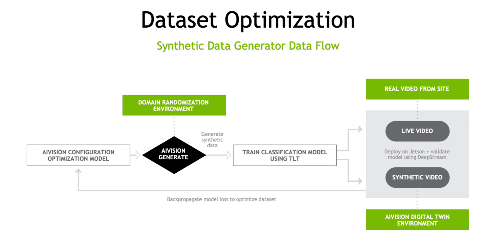
The synthetic data is then used to train a model that can be tested in a digital twin, a virtual representation of the warehouse, supply line, store, or whatever environment the model will be deployed. Using the synthetic data and the digital twin, Kinetic Vision can train, simulate, and re-train the model to achieve the required level of accuracy.
Figure 2. Dataset optimization using synthetic data and digital twin environment
Once the AI model has achieved the desired level of performance, it must be tested in the real world. This is where NVIDIA Fleet Command comes in. Fleet Command is a hybrid-cloud platform for deploying and managing AI models at the edge. The pre-trained model is simply loaded into the NGC catalog and then deployed on the edge system using the Fleet Command UI in just a few clicks. Once deployed at the edge, the model can continue to be optimized with real world data sent back from the store or warehouse. These updates are once again easily deployed and managed using Fleet Command.
The advantages of this new approach to creating retail computer vision applications include both ROI and technological benefits. The cost of developing an AI model with a digital twin is easily 10 percent the time and cost required to do the same thing in a physical environment. With the digital twin, testing can be done without physical infrastructure or requiring production interruptions. Additionally, new products and product variations can be easily accommodated without requiring inventory photography that must be manually annotated. Finally, the digital twin results in a generalized and scalable model that still provides the accuracy required for production deployment.
‘Meet the Researcher’ is a series in which we spotlight different researchers in academia who use NVIDIA technologies to accelerate their work. This month we spotlight Dr. Emanuel Gull, Associate Professor of Physics at University of Michigan, whose research focuses on the development of theoretical and computational methods for strongly correlated quantum systems. Gull is … Continued
‘Meet the Researcher’ is a series in which we spotlight different researchers in academia who use NVIDIA technologies to accelerate their work.
This month we spotlight Dr. Emanuel Gull, Associate Professor of Physics at University of Michigan, whose research focuses on the development of theoretical and computational methods for strongly correlated quantum systems.
Gull is the recipient of a Sloan Research Fellow, Ralph E. Powe Junior Faculty Enhancement Award, DOE Early Career Research Award, SCES early career Nevill F. Mott Prize, and APS Outstanding Referee Program.
What are your research areas?
The physics of materials in which many quantum particles strongly interact with each other. These are the systems out of which we build our newest generation of magnets, superconductors, solar cells, and systems for standard approximative methods.
When did you know that you wanted to be a researcher and pursue this field?
I was always open to having a career in the software/computing side of industry/finance — but, when I had to decide whether to go for a postdoc, the financial crisis hit. Instead, I did a postdoc in the U.S. and managed to get hired into an academic position afterwards.
What motivated you to pursue your recent research area of focus? ‘Quantum’ theory is the reason why many of our recent technological breakthroughs work. After all, NVIDIA chips are just an application of quantum theory. However, taking just theory and predicting and improving material properties without further input is incredibly difficult, even though we believe we understand the theory very well. I have always been fascinated by the challenge of combining computers and theoretical methods to bring calculations closer to reality. This started with an internship I did at a high performance computer center back when I was a high school student.
What problems or challenges does your research address?
While we know the equations that govern the physics of systems with many interacting quantum particles well, they are impossibly difficult to solve. This is why we need to find approximations that are both numerically tractable and accurate. My research spans the entire gamut from theoretical derivations, to implementation of new algorithms, to HPC, to comparisons with experiments. All of my research aims to make quantum theories more predictive and more accurate.
What challenges did you face during the research process, and how did you overcome them? Time management is probably the most crucial. It’s easy to have many ideas, but testing them, improving upon them, and revising them takes time. In research, you’re constantly juggling finding resources, training people, having and revising ideas, publishing, going to conferences, etc. Finding quiet intervals to work deeply on a problem is essential, but difficult. I don’t believe I’ve overcome that limitation.
What is the impact of your work on the field/community/world?
Stronger magnets, higher temperature superconductors, and better materials for sensors and chips.
How have you used NVIDIA technology either in your current or previous research?
Yes! In fact, our home-written ab-initio simulation toolkit uses NVIDIA codes to simulate the physics of real materials and their excitations. Most of our calculations would be either impossible or borderline without the NVIDIA fast and double-precision arithmetics on the V100 and A100. Our codes run at just about 50% of theoretical peak flop, and are parallelized with streams within each GPU and with MPI between different GPUs and nodes. What research breakthroughs or interesting results can you share?
We did, and we’re just now writing a paper on a new high-temperature superconductor.
What’s next for your research?
We’re currently doing a big push for driving systems out of equilibrium. We’re exciting them with a laser, ‘quenching’ them with a short current pulse, or probing them in other nonequilibrium conditions. The nonequilibriumphysics of quantum materials is very different from the equilibrium conditions, and many exciting new phenomena appear. Besides, most sensors work out of equilibrium. How to generalize our computational toolkit to these situations is currently an open question that we’re working on.
Any advice for new researchers, especially to those who are inspired and motivated by your work? Ask the big questions. Why is this interesting? Why will it work or how will it not work? What have we learned if it does work? But, don’t lose sight of the small details. Pounce at the details that don’t quite make sense, that’s where there’s something that needs to be understood. When something turns into a dead end, learn to let it go (even if you’ve invested a lot of resources into it).
Also, know the established ways of thinking about a problem, but question them always. Know the limitations of your tools and theories, and invest in your toolkit. New tools (computer codes, theoretical methods, experimental setups) lead to new discoveries, so make sure you have the best ones available for your application.
A pair of new demos running GeForce RTX technologies on the Arm platform unveiled by NVIDIA today show how advanced graphics can be extended to a broader, more power-efficient set of devices. The two demos, shown at this week’s Game Developers Conference, included Wolfenstein: Youngblood from Bethesda Softworks and MachineGames, as well as The Bistro Read article >
Top game artists, producers, developers and designers are coming together this week for the annual Game Developers Conference. As they exchange ideas, educate and inspire each other, the NVIDIA Studio ecosystem of RTX-accelerated apps, hardware and drivers is helping advance their craft. GDC 2021 marks a major leap in game development with NVIDIA RTX technology Read article >
Discover how NVIDIA CloudXR with Teradici’s PCoIP protocol enables XR users to experience seamless streaming. CloudXR uses Teradici’s ability to support high-fidelity video and use of flexible integration options for enterprise IT systems.
NVIDIA CloudXR is an SDK that enables you to implement real-time GPU rendering and streaming of rich VR, AR, and XR applications on remote servers, including the cloud. Applications can connect and stream remotely on low-powered VR devices or tablets where normally they wouldn’t function properly.
However, even when the underlying application executes on a remote NVIDIA CloudXR server, there are times when a facilitator wants to mirror the view of what an XR user sees. Unlike many consumer-driven experiences, enterprise XR applications often require a degree of synchronous interactivity between the user in XR and an external non-VR user.
To achieve connectivity to a NVIDIA CloudXR server for non-XR users, there are many methods available, each with their own considerations. Microsoft RDP supports a “headless” implementation of NVIDIA CloudXR by streaming XR content to a headset or tablet without requiring a host to log in to the server. However, this is not helpful in cases where a trainer or coach is needed to monitor the XR experience streamed to the headset. Virtual Network Computing (VNC), a popular alternative to RDP, must meet strict security requirements in enterprise environments. As such, it’s common for VNC connections to be prohibited.
It supports high-fidelity video and frame rate experiences for host connections.
It enables flexible integration options for enterprise IT requirements.
Deployment can also be orchestrated and streamlined to multiple cloud providers, making it seamless for most NVIDIA CloudXR-powered applications.
“Use of AR and VR is increasing, particularly for our customers in industries like AEC and Game Development. Collaborations, such as this initiative with NVIDIA, ensure that Teradici CAS provides the absolute best user experience for designers and engineers with the trusted security of PCoIP, which keeps proprietary designs safe in the cloud.”
Mirela Cunjalo, director of product management at Teradici
Teradici CAS offers a secure high-performance remote workstation user interface for the CAD designer or content creator developing 3D content, also streamed as a VR session either collaboratively or to the same design.
Teradici offers easy-to-consume marketplace instances for every major cloud provider. This creates a great baseline with a guest OS (Windows Server 2019), NVIDIA drivers and licensing, and the Teradici CAS Ultra software preinstalled.
You can install and configure NVIDIA CloudXR Server, SteamVR, and your favorite AR or VR application, and you’ll instantly have a powerful cloud workstation.
To get started, procure the preferred marketplace offer for Teradici, depending on your cloud service provider of choice:
Next, select an NVIDIA-powered instance type available from the cloud provider. Follow your organization’s networking and security best practices to ensure connectivity to your instances. Download a PCoIP client, based on the client OS, to start a session on the cloud instance. Finally, enter the IP addresses for your instances and define the username and password for the PCoIP client.
With NVIDIA CloudXR, you can further enhance immersive experiences and deliver advanced VR and AR sessions to untethered devices. For more information, see NVIDIA CloudXR.
RTXMU (RTX Memory Utility) combines both compaction and suballocation techniques to optimize and reduce memory consumption of acceleration structures for any DXR or Vulkan Ray Tracing application.
Acceleration structures spatially organize geometry to accelerate ray tracing traversal performance. When you create an acceleration structure, a conservative memory size is allocated.
Upon initial build, the graphics runtime doesn’t know how optimally a geometry fits into the oversized acceleration structure memory allocation.
After the build is executed on the GPU, the graphics runtime reports back the smallest memory allocation that the acceleration structure can fit into.
This process is called compacting the acceleration structure and it is important for reducing the memory overhead of acceleration structures.
Another key ingredient to reducing memory is suballocating acceleration structures. Suballocation enables acceleration structures to be tightly packed together in memory by using a smaller memory alignment than is required by the graphics API.
Typically, buffer allocation alignment is at a minimum of 64 KB while the acceleration structure memory alignment requirement is only 256 B. Games using many small acceleration structures greatly benefit from suballocation, enabling the tight packaging of many small allocations.
The NVIDIA RTX Memory Utility (RTXMU) SDK is designed to reduce the coding complexity associated with optimal memory management of acceleration structures. RTXMU provides compaction and suballocation solutions for both DXR and Vulkan Ray Tracing while the client manages synchronization and execution of acceleration structure building. The SDK provides sample implementations of suballocators and compaction managers for both APIs while providing flexibility for the client to implement their own version.
For more information about why compaction and suballocation are so important in reducing acceleration structure memory overhead, see Tips: Acceleration Structure Compaction.
Why Use RTXMU?
RTXMU allows you to quickly integrate acceleration structure memory reduction techniques into their game engine. Below is a summary of these techniques along with some key benefits in using RTXMU
Reduces the memory footprint of acceleration structures involves both compaction and suballocation code, which are not trivial to implement. RTXMU can do the heavy lifting.
Abstracts away memory management of bottom level acceleration structures (BLASes) but is also flexible enough to enable users to provide their own implementation based on their engine’s needs.
Manages all barriers required for compaction size readback and compaction copies.
Passes back handles to the client that refer to complex BLAS data structures. This prevents any mismanagement of CPU memory, which could include accessing a BLAS that has already been deallocated or doesn’t exist.
Can help reduce BLAS memory by up to 50%.
Gives the benefit of less translation lookaside buffer (TLB) misses by packing more BLASes into 64 KB or 4 MB pages.
RTXMU Design
RTXMU has a design philosophy that should reduce integration complexities for most developers. The key principles of that design philosophy are as follows:
All functions are thread-safe. If simultaneous access occurs, they are blocking.
The client passes in client-owned command lists and RTXMU populates them.
The client is responsible for synchronizing command list execution.
API Function Calls
RTXMU abstracts away the coding complexities associated with compaction and suballocation. The functions detailed in this section describe the interface entry points for RTXMU.
Initialize—Specifies the suballocator block size.
PopulateBuildCommandList—Receives an array of D3D12_BUILD_RAYTRACING_ACCELERATION_STRUCTURE_INPUTS and returns a vector of acceleration structure handles for the client to fetch acceleration structure GPUVAs later during top-level acceleration structure (TLAS) construction, and so on.
PopulateUAVBarriersCommandList – Receives acceleration structure inputs and places UAV barriers for them
PopulateCompactionSizeCopiesCommandList – Performs copies to bring over any compaction size data
PopulateUpdateCommandList—Receives an array of D3D12_BUILD_RAYTRACING_ACCELERATION_STRUCTURE_INPUTS and valid acceleration structure handles so that updates can be recorded.
PopulateCompactionCommandList—Receives an array of valid acceleration structure handles and records compaction commands and barriers.
RemoveAccelerationStructures—Receives an array of acceleration structure handles that specify which acceleration structure can be completely deallocated.
GarbageCollection—Receives an array of acceleration structure handles that specify that build resources (scratch and result buffer memory) can be deallocated.
GetAccelStructGPUVA—Receives an acceleration structure handle and returns a GPUVA of the result or compacted buffer based on state.
Reset—Deallocates all memory associated with current acceleration structure handles.
Suballocator DXR design
The BLAS suballocator works around the 64 KB and 4 MB buffer alignment requirement by placing small BLAS allocations within a larger memory heap. The BLAS suballocator still must fulfill the 256 B alignment required for BLAS allocations.
If the application requests 4 MB or larger suballocation blocks, then RTXMU uses placed resources with heaps that can provide 4 MB alignment.
If the application requests fewer than 4 MB suballocation blocks, then RTXMU uses committed resources, which only provide 64 KB alignment.
The BLAS suballocator reuses freed suballocations within blocks by maintaining a free list. If a memory request is greater than the suballocator block size, then a single allocation is created that can’t be suballocated.
Compaction DXR design
If the build requests compaction, then RTXMU requests that the compaction size be written out to a chunk of video memory. After the compaction size has been copied from video memory to system memory, then RTXMU allocates a suballocated compaction buffer to be used as the destination for the compaction copy.
The compaction copy takes the original build containing unused memory segments and truncates it down to the smallest memory footprint it can fit in. The original noncompacted build and scratch memory gets released back to the suballocator after compaction is complete. The only thing you have worry about is passing in the allow compaction flag and calling GetGPUVA with a BLAS handle. The GPUVA could either be the original build or the compacted build, based on what state the BLAS is in.
How to Use RTXMU
In this section, I detail the RTXMU sequence loop and synchronization.
RTXMU sequence loop
Figure 1 shows a normal usage pattern of RTXMU. The client manages the command list execution, while everything else is a call into RTXMU
First, initialize RTXMU by passing in the suballocator block size and the device responsible for allocating suballocation blocks. In each frame, the engine builds new acceleration structures while also compacting acceleration structures built in previous frames.
After RTXMU populates the client’s command lists, the client is free to execute and manage the synchronization of the initial build to the final compaction copy build. It’s important to make sure that each acceleration structure build has been fully executed before calling PopulateCompactionCommandList. This is left to the client to manage properly.
When an acceleration structure has finally reached the compaction state, then the client can choose to call GarbageCollection, which notifies RTXMU that the scratch and original acceleration structure buffer can be deallocated. If the engine does heavy streaming of assets, then the client can deallocate all acceleration structure resources by calling RemoveAS with a valid acceleration structure handle.
Figure 1. RTXMU flow chart of a typical use case delineating client and RTXMU code
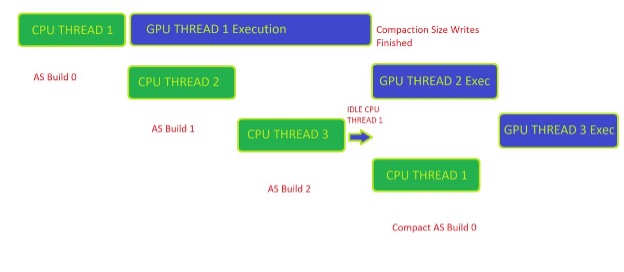
Figure 2 shows the synchronization required by the client to manage compaction-ready workloads properly. The example here is a triple frame buffered loop in which the client can have up to three asynchronous frames being built on the CPU and executed on the GPU.
To get the compaction size available on the CPU side, Build 0 must have finished executing on the GPU. After the client has received a fence signal back from the GPU, the client can then call RTXMU to start the compaction command list recording.
A helpful way to manage the synchronization of compaction for acceleration structures is to employ a key/value pair data structure of some kind that tracks the state of each acceleration structure handle given by RTXMU. The four basic states of an acceleration structure can be described as follows:
Prebuilt—The build command is recorded on a command list but hasn’t finished executing on the GPU.
Built— The initial build has been executed on the GPU and is ready for compaction commands.
Compacted—The compaction copy has been finished on the GPU and is ready for GarbageCollection to release the scratch and initial build buffers.
Released—The client releases the acceleration structure from memory because it is no longer in the scene. At that point, all memory associated with an acceleration structure handle is freed back to the OS.
Figure 2. Client code can only initiate compaction workloads after the initial acceleration structures builds have finished execution on the GPU.
RTXMU Test Scenes
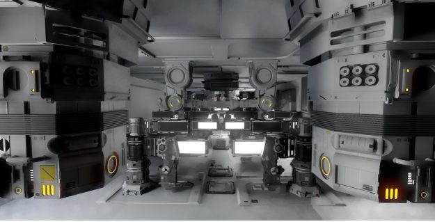
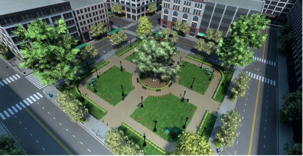
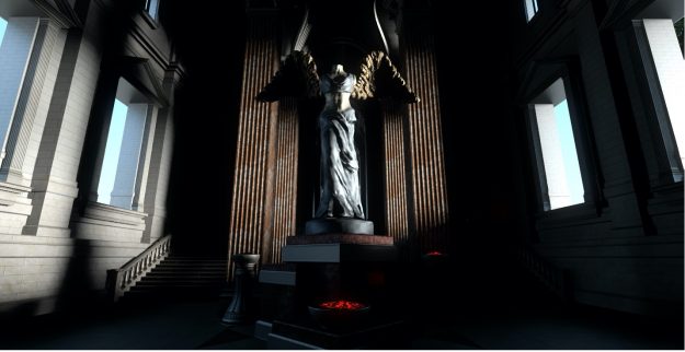
RTXMU was tested with six text scenes to provide real use case data about the benefits of compaction and suballocation. The following figures show just some of the scenes.
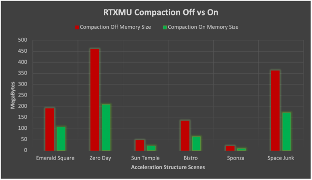
Figure 3. Zero Day scene 10,740 BLAS, uncompacted acceleration structure memory size 458.9 MB, compacted acceleration structure memory size 208.3 MB, 55% memory reduction, suballocating memory saved 71.3 MB
On average, compaction on NVIDIA RTX cards reduced acceleration structure by 52% for the test scenes. The standard deviation of compaction memory reduction was 2.8%, which is quite stable.
Figure 6. Bar graph comparing compaction on versus off on NVIDIA RTX 3000 series GPUs
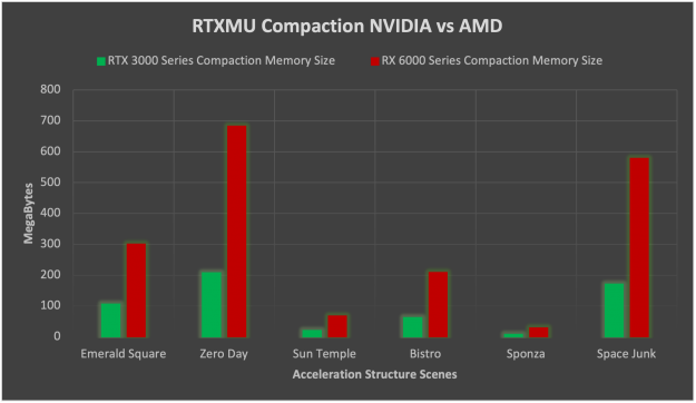
When enabling compaction on NVIDIA and AMD HW, the memory savings on NVIDIA HW is much improved compared to AMD. NVIDIA ends up being on average 3.26x smaller than AMD for acceleration structure memory when enabling compaction. The reason for such a huge reduction in memory footprint on NVIDIA is that AMD without compaction uses double the memory as is when compared to NVIDIA. Compaction then also reduces the NVIDIA memory by another 50% on average while AMD tends to reduce memory only by 75%.
Figure 7. Bar graph comparing compaction of NVIDIA 3000 series versus AMD 6000 series GPUs
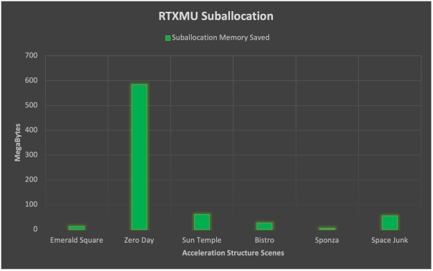
Suballocation tells a slightly different story here in which scenes with many small acceleration structures like Zero Day benefit greatly. The average memory savings from suballocation ends up being 123 MB but the standard deviation is rather large at 153 MB. From this data, we can assert that suballocation is highly dependent on the scene geometry and benefits from thousands of small triangle count BLAS geometry.
Figure 8. Bar graph showing the memory savings of suballocation for specific scenes
Source Code
NVIDIA is open-sourcing the RTXMU SDK along with a sample application integrating RTXMU. Maintaining RTXMU as an open-source project on GitHub helps developers understand the logic flow and provides access to modifying the underlying implementation. The RT Bindless sample application provides an example of an RTXMU integration for both Vulkan Ray Tracing and DXR backends.
Here’s how to build and run the sample application integrating RTXMU. You must have the following resources:
Windows, Linux, or an OS that supports DXR or Vulkan Ray Tracing
CMake 3.12
C++ 17
Git
First, clone the repository using the following command:
Next, open CMake. For Where is the source code, enter the /donut_examples folder. Create a build folder in the /donut_examples folder. For Where to build the binaries, enter the new build folder. Select the cmake variable NVRHI_WITH_RTXMU to ON, choose Configure, wait for it to complete and then click Generate.
If you are building with Visual Studio, then select 2019 and x64version. Open the donut_examples.sln file in Visual Studio and build the entire project.
Find the rt_bindless application folder under /Examples/Bindless Ray Tracing, choose the project context (right-click) menu, and choose Startup Project.
By default, bindless ray tracing runs on DXR. To run the Vulkan version, add -vk as a command-line argument in the project.
Summary
RTXMU combines both compaction and suballocation techniques to optimize and reduce memory consumption of acceleration structures for any DXR or Vulkan Ray Tracing application. The data shows that using RTXMU significantly reduces acceleration structure memory. This enables you to either add more geometry to your ray-traced scenes or use the extra memory for other resources.
Real-time ray tracing has advanced the art of lighting in video games, but it’s a computationally expensive process. Aiming to reduce these costs, NVIDIA has developed a memory utility that combines both compaction and suballocation techniques to optimize and reduce memory consumption of acceleration structures.
RTX Memory Utility (RTXMU) Available Now
Reducing Memory Consumption with an Open Source Solution
Real-time ray tracing has advanced the art of lighting in video games, but it’s a computationally expensive process. Aiming to reduce these costs, NVIDIA has developed a memory utility that combines both compaction and suballocation techniques to optimize and reduce memory consumption of acceleration structures. We’ve turned this solution into an SDK called RTXMU, and we are making it available as an open source release today. It’s built to support any DXR or Vulkan Ray Tracing application.
Compaction of acceleration structures with RTXMU eliminates any wasted memory from the initial build operation. For applications using RTXMU, NVIDIA RTX cards get a ~50% reduction in memory footprint. Additionally, suballocating acceleration structure buffers with RTXMU prevents fragmentation and wasted space. Scenes with thousands of small unique BLAS benefit greatly from suballocation.
How Can RTXMU Help You, Right Away?
RTXMU is easy to integrate, and it provides benefits immediately.
A suballocation and compaction memory manager takes significant engineering time to validate. RTXMU reduces the time it takes for a developer to integrate compaction and suballocation into an RTX title.
RTXMU also abstracts away the memory and compaction state management of the BLAS, and manages all barriers required for compaction size readback and compaction copies.
Diving a bit deeper, RTXMU uses handle indirection to BLAS data structures to prevent any mismanagement of CPU memory, which could include accessing a BLAS that has already been deallocated or doesn’t exist. Also, suballocation gives the benefit of less TLB (Translation Lookaside Buffer) misses by packing more BLASes into 64 KB or 4 MB pages.
Put simply, RTXMU will make your real-time ray traced games and applications run better, without significant effort on your part.
Where can I get RTXMU?
RTXMU is an open source SDK available today, and an update will come this week. For tips on deployment, check out our RTXMU getting started blog.
Nsight Graphics 2021.3 is an all-in-one graphics debugger and profiler to help game developers get the most out of NVIDIA hardware.
Nsight Graphics 2021.3 is an all-in-one graphics debugger and profiler to help game developers get the most out of NVIDIA hardware. From analyzing API setup to solve nasty bugs, to providing deep insight into how your application utilizes the GPU to drain every last bit of performance, Nsight Graphics is the ultimate tool in your arsenal.
We enhanced GPU Trace to support Vulkan/OpenGL interoperability. It is now possible for you to use the latest profiling capabilities on applications that use both the OpenGL and Vulkan graphics APIs. We support capturing OpenGL SwapBuffers calls for overall frame timing, as well as capturing screenshots of windows rendered to by OpenGL. You can also use NVTX to mark user ranges while using OpenGL.
We have enabled Optix support for GPU Trace, including Vulkan applications that trace rays in the compute shader and use OptiX as a denoiser. GPU Trace is able to show NVTX markers, which when used with OptiX can provide helpful contextual information. See NVIDIA OptiX Ray Tracing Engine for more information on OptiX.
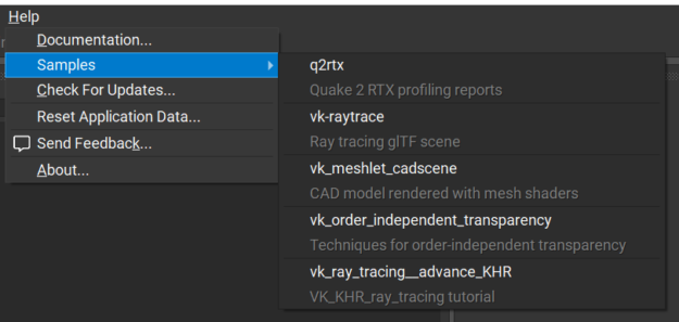
Nsight Graphics now ships with sample applications and reports to help you experiment with and understand many of the tool’s features. You can access them via the new Samples submenu menu in the top level Help menu.
The System Trace activity can now directly launch Nsight Systems from Nsight Graphics. This allows you to more easily utilize the powerful CPU and GPU profiling capabilities of Nsight Systems with the same application settings used by Nsight Graphics. Direct launch simplifies parameter management by allowing you to keep these application settings in a single location. This feature is compatible with Nsight Systems version 2021.3 or later.
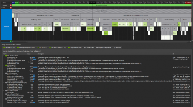
We have made improvements to the user interface for GPU Trace Analysis by changing the meaning of the severity and certainty icons. The original numeric groups have been refined, and we now use numbers or the ‘+’ icon to denote ranges with potential performance improvements. Further, these indicators scale according to the maximum projected gain, making it easier to find the most important ranges to focus on. All the detailed performance information is sorted and grouped in the tabs below the indicators, and provides a useful explanation of the metric evaluation suggestions, as well as steps to take to improve the performance of the range.
We have added the ability to rename a C++ Capture in the Project Explorer. This allows you to better organize or mark-up your C++ Captures.
Finally, we also added support for Arch Linux and the DirectX 12 Agility SDK
For more details on Nsight Graphics 2021.3, check out the release notes (link). Visit Nsight Graphics to stay informed about the latest updates.
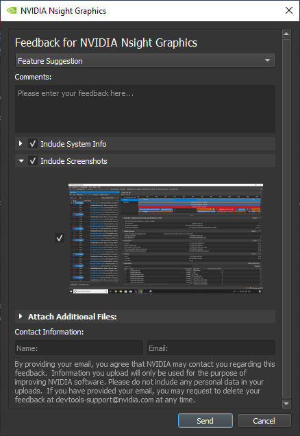
We want to hear from you! Please continue to use the integrated feedback button that lets you send comments, feature requests, and bugs directly to us with the click of a button. You can send feedback anonymously or provide an email so we can follow up with you about your feedback. Just click on the little speech bubble at the top right of the window.
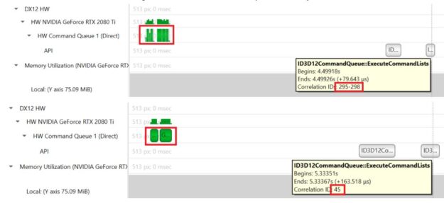
This release introduces several improvements aimed to assist the user with locating issues and improve the profiling experience. User workflows are improved with both the introduction of the Expert System View which identifies problematic patterns, as well as the new ability to load multiple reports into the same timeline to investigate multi-process issues with greater ease. Nsight Systems now supports Windows 21H1 SDK, sample GPU PCIe BAR1 request activity, trace UCX asynchronous API calls, and trace Vulkan QueueSubmit or Direct3D12 ExecuteCommandList GPU workloads as a reduced overhead option.
Fig 1. GPU PCIe BAR1 request activity
Fig 2. Batch command-buffers/command-lists trace
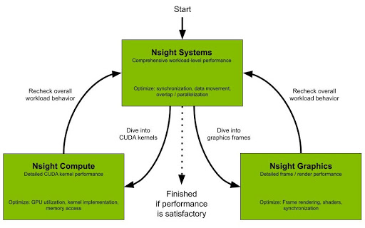
Nsight Systems is part of a larger family of Nsight tools. A developer can start with Nsight Systems to see the big picture and avoid picking less efficient optimizations based on assumptions and false-positive indicators.
NVIDIA has made Deep Learning Super Sampling (DLSS) easier and more flexible than ever for developers to access and integrate in their games. The latest DLSS SDK update (version 2.2.1) enables new user customizable options, delivers Linux support and streamlines access.
Today, NVIDIA has made Deep Learning Super Sampling (DLSS) easier and more flexible than ever for developers to access and integrate in their games. The latest DLSS SDK update (version 2.2.1) enables new user customizable options, delivers Linux support and streamlines access.
NVIDIA DLSS technology has already been adopted and implemented in over 60 games, including the biggest gaming franchises such as Cyberpunk, Call of Duty, DOOM, Fortnite, LEGO, Minecraft,Rainbow Six, and Red Dead Redemption, with support coming soon for Battlefield 2042. DLSS uses the power of RTX Tensor Cores to boost game frame rates through an advanced deep learning temporal super resolution algorithm.
New User & Developer Customizable Options
This DLSS update offers new options to developers during the integration process. A new sharpening slider allows users to make an image sharper or softer based on their own personal preferences. DLSS Auto Mode enables optimal image quality for a particular resolution. For resolutions at or under 1440P, DLSS Auto is set to Quality, 4K set to Performance, and 8K set to Ultra Performance. Lastly, an auto-exposure option offers an automatic way to calculate exposure values for developers. This option can potentially improve the image quality of low-contrast scenes.
Linux Support Available Now
Last month, NVIDIA added DLSS support for Vulkan API games on Proton, enabling Linux gamers to boost frame rates on Proton-supported titles such as DOOM Eternal, No Man’s Sky, and Wolfenstein: Youngblood. Today, the NVIDIA DLSS SDK is adding support for games running natively on Linux with x86. We are also announcing DLSS support for ARM-based platforms.
Easier Access for Developers
Accessing the DLSS SDK is now easier than ever — no application required! Simply download the DLSS SDK 2.2.1 directly from the NVIDIA Developer website, access the Unreal Engine 5 and 4.26 plugin from the marketplace, or utilize DLSS natively in Unity 2021.2 beta.
Make sure to tune into the NVIDIA DLSS virtual session at Game Developers Conference (GDC) July 19 – 23 to learn about best practices on integrating DLSS into your game. And check out the latest DLSS game releases here.

 A new session from GTC shares how to use synthetic data and Fleet Command to deploy highly accurate and scalable models.
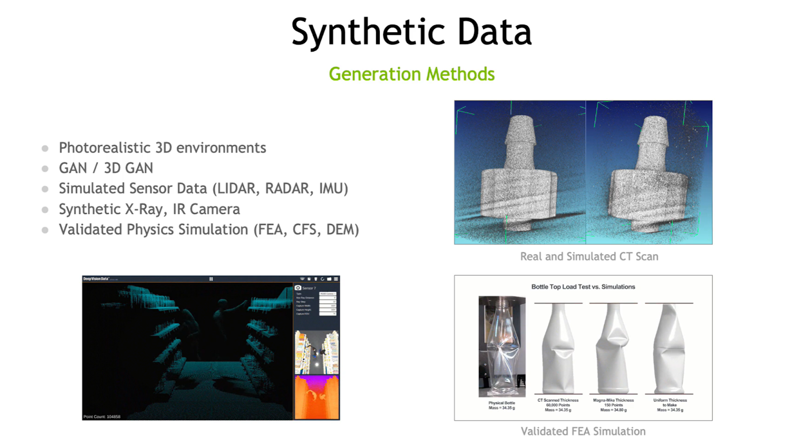
 ‘Meet the Researcher’ is a series in which we spotlight different researchers in academia who use NVIDIA technologies to accelerate their work. This month we spotlight Dr. Emanuel Gull, Associate Professor of Physics at University of Michigan, whose research focuses on the development of theoretical and computational methods for strongly correlated quantum systems. Gull is …
  Discover how NVIDIA CloudXR with Teradici’s PCoIP protocol enables XR users to experience seamless streaming. CloudXR uses Teradici’s ability to support high-fidelity video and use of flexible integration options for enterprise IT systems.
 RTXMU (RTX Memory Utility) combines both compaction and suballocation techniques to optimize and reduce memory consumption of acceleration structures for any DXR or Vulkan Ray Tracing application.
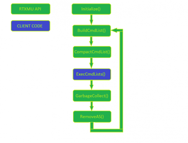
 Real-time ray tracing has advanced the art of lighting in video games, but it’s a computationally expensive process. Aiming to reduce these costs, NVIDIA has developed a memory utility that combines both compaction and suballocation techniques to optimize and reduce memory consumption of acceleration structures.
 Nsight Graphics 2021.3 is an all-in-one graphics debugger and profiler to help game developers get the most out of NVIDIA hardware.
 support for GPU Trace, including Vulkan applications that trace rays in the compute shader and use OptiX
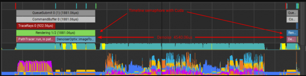
 Nsight Systems is a system-wide performance analysis tool, designed to help developers tune and scale software across CPUs and GPUs.
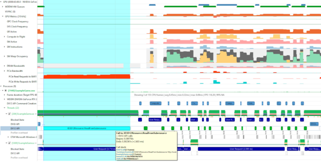
 NVIDIA has made Deep Learning Super Sampling (DLSS) easier and more flexible than ever for developers to access and integrate in their games. The latest DLSS SDK update (version 2.2.1) enables new user customizable options, delivers Linux support and streamlines access.