DataBloom

submitted by /u/WhoKnows2019
[visit reddit] [comments]

submitted by /u/KIProf
[visit reddit] [comments]

Speech is the most natural form of human communication. So, it’s not surprising that we’ve always wanted to interact with and command machines by voice. However, for conversational AI to provide a seamless, natural, and human-like experience, it needs to be trained on large amounts of data representative of the problem the model is trying … Continued

Speech is the most natural form of human communication. So, it’s not surprising that we’ve always wanted to interact with and command machines by voice. However, for conversational AI to provide a seamless, natural, and human-like experience, it needs to be trained on large amounts of data representative of the problem the model is trying to solve. The difficulty for machine learning teams is the scarcity of this high-quality, domain-specific data.

Companies are trying to solve this problem and accelerate the widespread adoption of conversational AI with innovative solutions that guarantee the scalability and internationality of models. NVIDIA and DefinedCrowd are two such companies. By providing machine learning engineers with a model-building toolkit and high-quality training data respectively, NVIDIA and DefinedCrowd integrate to create world-class AI simply, easily, and quickly.

DefinedCrowd, a one-stop shop for AI training data

I am the director of machine learning at DefinedCrowd, and our core business is providing high-quality AI training data to companies building world-class AI solutions. Our customers can access this data through DefinedData, an online marketplace of off-the-shelf AI training data available in multiple languages, domains, and recording types.

If you can’t find what you’re looking for in DefinedData, our workflows can serve as standalone or end-to-end data services to build any speech– or text-enabled AI architecture from scratch, to improve solutions already developed, or to evaluate models in production, all with the DefinedCrowd quality guarantee.

Creating conversational AI applications the easy way

NVIDIA NeMo is a toolkit built by NVIDIA for creating conversational AI applications. This toolkit includes collections of pretrained modules for automatic speech recognition (ASR), natural language processing (NLP), and text-to-speech (TTS), enabling researchers and data scientists to easily compose complex neural network architectures and focus on designing their applications.

NeMo and DefinedCrowd integration

Here’s how to connect DefinedCrowd speech workflows to train and improve an ASR model using NVIDIA NeMo.  The code can also be accessed on this Google Colab link.

Step 1: Install NeMo Toolkit and dependencies

# First, install NeMo Toolkit and dependencies to run this notebook
!apt-get install -y libsndfile1 ffmpeg
!pip install Cython

## Install NeMo dependencies in the correct versions
!pip install torchtext==0.8.0 torch==1.7.1 pytorch-lightning==1.2.2

## Install NeMo
!python -m pip install nemo_toolkit[all]==1.0.0b3

Step 2: Obtain data using the DefinedCrowd API

Here’s how to connect to the DefinedCrowd API to obtain speech collected data. For more information, see DefinedCrowd API (v2).

# For the demo, use a sandbox environment
auth_url = "https://sandbox-auth.definedcrowd.com"
api_url = "https://sandbox-api.definedcrowd.com"

# These variables should be obtained at the DefinedCrowd Enterprise Portal for your account.
client_id = ""
client_secret = ""
project_id = ""

Authentication

payload = {
    "client_id": client_id,
    "client_secret": client_secret,
    "grant_type": "client_credentials",
    "scope": "PublicAPIv2",
}
files = []
headers = {}

# request the Auth 2.0 access token
response = requests.request(
    "POST", f"{auth_url}/connect/token", headers=headers, data=payload, files=files
)
if response.status_code == 200:
    print("Authentication success!")
    access_token = response.json()["access_token"]
else:
    print("Authentication Failed")

Authentication success!

List of deliverables

# GET /projects/{project-id}/deliverables
headers = {"Authorization": "Bearer " + access_token}
response = requests.request(
    "GET", f"{api_url}/projects/{project_id}/deliverables", headers=headers
)

if response.status_code == 200:
    # Pretty print the response
    print(json.dumps(response.json(), indent=4))

    # Get the first deliverable ID
    deliverable_id = response.json()[0]["id"]

[
    {
        "projectId": "eb324e45-c4f9-41e7-b5cf-655aa693ae75",
        "id": "258f9e15-2937-4846-b9c3-3ae1164b7364",
        "type": "Flat",
        "fileName": "data_Flat_eb324e45-c4f9-41e7-b5cf-655aa693ae75_258f9e15-2937-4846-b9c3-3ae1164b7364_2021-03-22-14-34-37.zip",
        "createdTimestamp": "2021-03-22T14:34:37.8037259",
        "isPartial": false,
        "downloadCount": 2,
        "status": "Downloaded"
    }
]

Final deliverable for speech data collection

# Name to give to the deliverable file
filename = "scripted_monologue_en_GB.zip"

# GET /projects/{project-id}/deliverables/{deliverable-id}/download
headers = {"Authorization": "Bearer " + access_token}
response = requests.request(
    "GET",
    f"{api_url}/projects/{project_id}/deliverables/{deliverable_id}/download/",
    headers=headers,
)

if response.status_code == 200:
    # save the deliverable file
    with open(filename, "wb") as fp:
        fp.write(response.content)
    print("Deliverable file saved with success!")

Deliverable file saved with success!

# Extract the contents from the downloaded file
!unzip  scripted_monologue_en_GB.zip &> /dev/null
!rm -f en-gb_single-scripted_Dataset.zip

Step 3: Analyze the speech dataset

Here’s how to analyze the data received from DefinedCrowd. The data is built of scripted speech data collected by the DefinedCrowd Neevo platform from several speakers in the UK (crowd members from DefinedCrowd).

Each row of the dataset contains information about the speech prompt, crowd member, device used, and the recording. The following data is found with this delivery:

• Recording:
  • RecordingId
  • PromptId
  • Prompt
• Audio File:
  • RelativeFileName
  • Duration
  • SampleRate
  • BitDepth
  • AudioCommunicationBand
  • RecordingEnvironment
• Crowd Member:
  • SpeakerId
  • Gender
  • Age
  • Accent
  • LivingCountry
• Recording Device:
  • Manufacturer
  • DeviceType
  • Domain

This data can be used for multiple purposes, but in this tutorial, I use it for improving an existent ASR model for British speakers.

import pandas as pd

# Look in the metadata file
dataset = pd.read_csv("metadata.tsv", sep="t", index_col=[0])

# Check the data for the first row
dataset.iloc[0]

RecordingId                               165559628
PromptId                                   64977250
RelativeFileName                Audio/165559628.wav
Prompt                    The Avengers' extinction.
Duration                               00:00:02.815
SpeakerId                                    128209
Gender                                       Female
Age                                              26
Manufacturer                                  Apple
DeviceType                                iPhone 6s
Accent                                      Suffolk
Domain                                      generic
SampleRate                                    16000
BitDepth                                         16
AudioCommunicationBand                    Broadband
LivingCountry                        United Kingdom
Native                                         True
RecordingEnvironment                         silent
Name: 0, dtype: object

# How many rows do you have?
len(dataset)

50000

# Check some examples from the dataset
import librosa
import IPython.display as ipd

for index, row in dataset.sample(4, random_state=1).iterrows():

    print(f"Prompt: {dataset.iloc[index].Prompt}")
    audio_file = dataset.iloc[index].RelativeFileName

    # Load and listen to the audio file
    audio, sample_rate = librosa.load(audio_file)
    ipd.display(ipd.Audio(audio, rate=sample_rate))

For audio samples, see the DefinedCrowd x NeMo – ASR Training tutorial on Google Colab.

Step 4: Prepare the data

After downloading the speech data from DefinedCrowd API, you must adapt it for the format expected by NeMo for ASR training. For this, you create manifests for the training and evaluation data, including each audio file’s metadata.

NeMo requires that you adapt the data to a particular manifest format. Each line corresponding to one audio sample, so the line count equals the number of samples represented by the manifest. A line must contain the path to an audio file, the corresponding transcript, and the audio sample duration. For example, here is what one line might look like in a NeMo-compatible manifest:

{"audio_filepath": "path/to/audio.wav", "duration": 3.45, "text": "this is a nemo tutorial"}

For the creation of the manifest, also standardize the transcripts.

import os

# Function to build a manifest
def build_manifest(dataframe, manifest_path):
    with open(manifest_path, "w") as fout:
        for index, row in dataframe.iterrows():
            transcript = row["Prompt"]

            # The model uses lowercased data for training/testing
            transcript = transcript.lower()

            # Removing linguistic marks (they are not necessary for this demo)
            transcript = (
                transcript.replace("", "")
                .replace("", "")
                .replace("[b_s/]", "")
                .replace("[uni/]", "")
                .replace("[v_n/]", "")
                .replace("[filler/]", "")
                .replace('"', "")
                .replace("[n_s/]", "")
            )

            audio_path = row["RelativeFileName"]

            # Get the audio duration
            try:
                duration = librosa.core.get_duration(filename=audio_path)
            except Exception as e:
                print("An error occurred: ", e)

            if os.path.exists(audio_path):
                # Write the metadata to the manifest
                metadata = {
                    "audio_filepath": audio_path,
                    "duration": duration,
                    "text": transcript,
                }
                json.dump(metadata, fout)
                fout.write("n")
            else:
                continue

Step 5: Train and test splits

To test the quality of the model, you must reserve some data for model testing. Evaluate the model performance on this data.

import json
from sklearn.model_selection import train_test_split
# Split 10% for testing (500 prompts) and 90% for training (4500 prompts)
trainset, testset = train_test_split(dataset, test_size=0.1, random_state=1)
# Build the manifests
build_manifest(trainset, "train_manifest.json")
build_manifest(testset, "test_manifest.json")

Step 6: Configure the model

Here’s how to use the QuartzNet15x5 model as a base model for fine-tuning with the data. To improve the recognition of the dataset, benchmark the model performance on the base model and later, on the fine-tuned version. Some of the following functions were retrieved from the Nemo Tutorial on ASR.

# Import Nemo and the functions for ASR
import torch
import nemo
import nemo.collections.asr as nemo_asr
import logging
from nemo.utils import _Logger
# Set up the log level by NeMo
logger = _Logger()
logger.set_verbosity(logging.ERROR)

Step 7: Set training parameters

For training, NeMo uses a Python dictionary as data structure to keep all the parameters. For more information, see the NeMo ASR Config User Guide.

For this tutorial, load a preexisting file with the standard ASR configuration and change only the necessary fields.

## Download the config to use in this example
!mkdir configs
!wget -P configs/ https://raw.githubusercontent.com/NVIDIA/NeMo/main/examples/asr/conf/config.yaml &> /dev/null

# --- Config Information ---#
from ruamel.yaml import YAML

config_path = "./configs/config.yaml"

yaml = YAML(typ="safe")
with open(config_path) as f:
    params = yaml.load(f)

Step 8: Download the base model

For the ASR model, use a pretrained QuartzNet15x5 model from the NGC catalog.

QuartzNet15x5 model trained on six datasets: LibriSpeech, Mozilla Common Voice (validated clips from en_1488h_2019-12-10), WSJ, Fisher, Switchboard, and NSC Singapore English. It was trained with Apex/Amp optimization level O1 for 600 epochs. The model achieves a WER of 3.79% on LibriSpeech dev-clean, and a WER of 10.05% on dev-other.

# This line downloads the pretrained QuartzNet15x5 model from NGC and instantiates it for you
quartznet = nemo_asr.models.EncDecCTCModel.from_pretrained(model_name="QuartzNet15x5Base-En", strict=False)

Step 9: Evaluate the base model performance

The word error rate (WER) is a valuable measurement tool for comparing different ASR model and evaluating improvements within one system. To obtain the results, assess how the model performs by using the testing set.

# Configure the model parameters for testing

# Parameters for training, validation, and testing are specified using the 
# train_ds, validation_ds, and test_ds sections of your configuration file

# Bigger batch-size = bigger throughput
params["model"]["validation_ds"]["batch_size"] = 8

# Set up the test data loader and make sure the model is on GPU
params["model"]["validation_ds"]["manifest_filepath"] = "test_manifest.json"
quartznet.setup_test_data(test_data_config=params["model"]["validation_ds"])

# Comment out this line if you don't want to use GPU acceleration
_ = quartznet.cuda()

# Compute the WER metric between the hypothesis and predictions.

wer_numerators = []
wer_denominators = []

# Loop over all test batches.
# Iterating over the model's `test_dataloader` gives you:
# (audio_signal, audio_signal_length, transcript_tokens, transcript_length)
# See the AudioToCharDataset for more details.
with torch.no_grad():
    for test_batch in quartznet.test_dataloader():
        input_signal, input_signal_length, targets, targets_lengths = [x.cuda() for x in test_batch]
                
        log_probs, encoded_len, greedy_predictions = quartznet(
            input_signal=input_signal, 
            input_signal_length=input_signal_length
        )
        # The model has a helper object to compute WER
        quartznet._wer.update(greedy_predictions, targets, targets_lengths)
        _, wer_numerator, wer_denominator = quartznet._wer.compute()
        wer_numerators.append(wer_numerator.detach().cpu().numpy())
        wer_denominators.append(wer_denominator.detach().cpu().numpy())

# First, sum all numerators and denominators. Then, divide.
print(f"WER = {sum(wer_numerators)/sum(wer_denominators)*100:.2f}%")

WER = 39.70%

Step 10: Fine-tune the model

The base model got 39.7% of WER, which is not so good. Maybe providing some data from the same domain and language dialects can improve the ASR model. For simplification, train for only one epoch using DefinedCrowd’s data.

import pytorch_lightning as pl
from omegaconf import DictConfig
import copy

# Before training, you must provide the train manifest for training
params["model"]["train_ds"]["manifest_filepath"] = "train_manifest.json"

# Use the smaller learning rate for fine-tuning
new_opt = copy.deepcopy(params["model"]["optim"])
new_opt["lr"] = 0.001
quartznet.setup_optimization(optim_config=DictConfig(new_opt))

# Batch size depends on the GPU memory available
params["model"]["train_ds"]["batch_size"] = 8

# Point to the data to be used for fine-tuning as the training set
quartznet.setup_training_data(train_data_config=params["model"]["train_ds"])

# Clean the torch cache
torch.cuda.empty_cache()

# Now you can create a PyTorch Lightning trainer.
trainer = pl.Trainer(gpus=1, max_epochs=1)

# The fit function starts the training
trainer.fit(quartznet)

Step 11: Compare model performance

Compare the final model performance with the fine-tuned model that you received from training with additional data.

# Configure the model parameters for testing
params["model"]["validation_ds"]["batch_size"] = 8

# Set up the test data loader and make sure the model is on GPU
params["model"]["validation_ds"]["manifest_filepath"] = "test_manifest.json"
quartznet.setup_test_data(test_data_config=params["model"]["validation_ds"])
_ = quartznet.cuda()

# Compute the WER metric between the hypothesis and predictions.

wer_numerators = []
wer_denominators = []

# Loop over all test batches.
# Iterating over the model's `test_dataloader` gives you:
# (audio_signal, audio_signal_length, transcript_tokens, transcript_length)
# See the AudioToCharDataset for more details.
with torch.no_grad():
    for test_batch in quartznet.test_dataloader():
        input_signal, input_signal_length, targets, targets_lengths = [x.cuda() for x in test_batch]
                
        log_probs, encoded_len, greedy_predictions = quartznet(
            input_signal=input_signal, 
            input_signal_length=input_signal_length
        )
        # The model has a helper object to compute WER
        quartznet._wer.update(greedy_predictions, targets, targets_lengths)
        _, wer_numerator, wer_denominator = quartznet._wer.compute()
        wer_numerators.append(wer_numerator.detach().cpu().numpy())
        wer_denominators.append(wer_denominator.detach().cpu().numpy())

# First, sum all numerators and denominators. Then, divide.
print(f"WER = {sum(wer_numerators)/sum(wer_denominators)*100:.2f}%")

WER = 24.36%

After training new epochs of the neural network ASR architecture, I achieved a WER of 24.36%, which is an improvement over the initial 39.7% from the base model using only one epoch for training. For better results, consider using more epochs in the training.

Conclusion

In this tutorial, I demonstrated how to load speech data collected by DefinedCrowd and how to use it to train and measure the performance of an ASR model. I hope I have shown you how easy it is to create world-class AI solutions with NVIDIA and DefinedCrowd.

High-energy physics research aims to understand the mysteries of the universe by describing the fundamental constituents of matter and the interactions between them. Diverse experiments exist on Earth to re-create the first instants of the universe. Two examples of the most complex experiments in the world are at the Large Hadron Collider (LHC) at CERN … Continued

High-energy physics research aims to understand the mysteries of the universe by describing the fundamental constituents of matter and the interactions between them. Diverse experiments exist on Earth to re-create the first instants of the universe. Two examples of the most complex experiments in the world are at the Large Hadron Collider (LHC) at CERN and the Deep Underground Neutrino Experiment (DUNE) at Fermilab.

The LHC is home to the highest energy particle collisions in the world and the discovery of the Higgs boson. LHC detectors are like ultra–high-speed cameras that capture the remnants of those collisions every 25 nanoseconds to create a 5D image in space, time, and energy. LHC physicists collect huge datasets to find extremely rare events. Those events may give clues about the Higgs boson as a portal to new physics or the particle nature of dark matter.

The DUNE experiment sends a beam of particles called neutrinos from the west suburbs of Chicago to an underground mine 1,300 km away in South Dakota. There, a massive 40-kton detector is being constructed 1.5 km beneath the earth’s surface to observe these feebly interacting particles. Studying neutrinos can help us answer questions such as the origin of matter in the universe and the behavior of core-collapse supernova in the Milky Way galaxy.

These experiments consist of unique and cutting-edge particle detectors that create massive, complex, and rich datasets with billions of events. They require sophisticated algorithms to reconstruct and interpret the data.

Modern machine learning algorithms provide a powerful toolset to detect and classify particles, from familiar image-processing convolutional neural networks to newer graph neural network architectures. A full reconstruction of these particle collisions requires novel approaches to handle the computing challenge of processing so much raw data. In a series of studies, physicists from Fermilab, CERN, and university groups explored how to accelerate their data processing using NVIDIA Triton Inference Server.

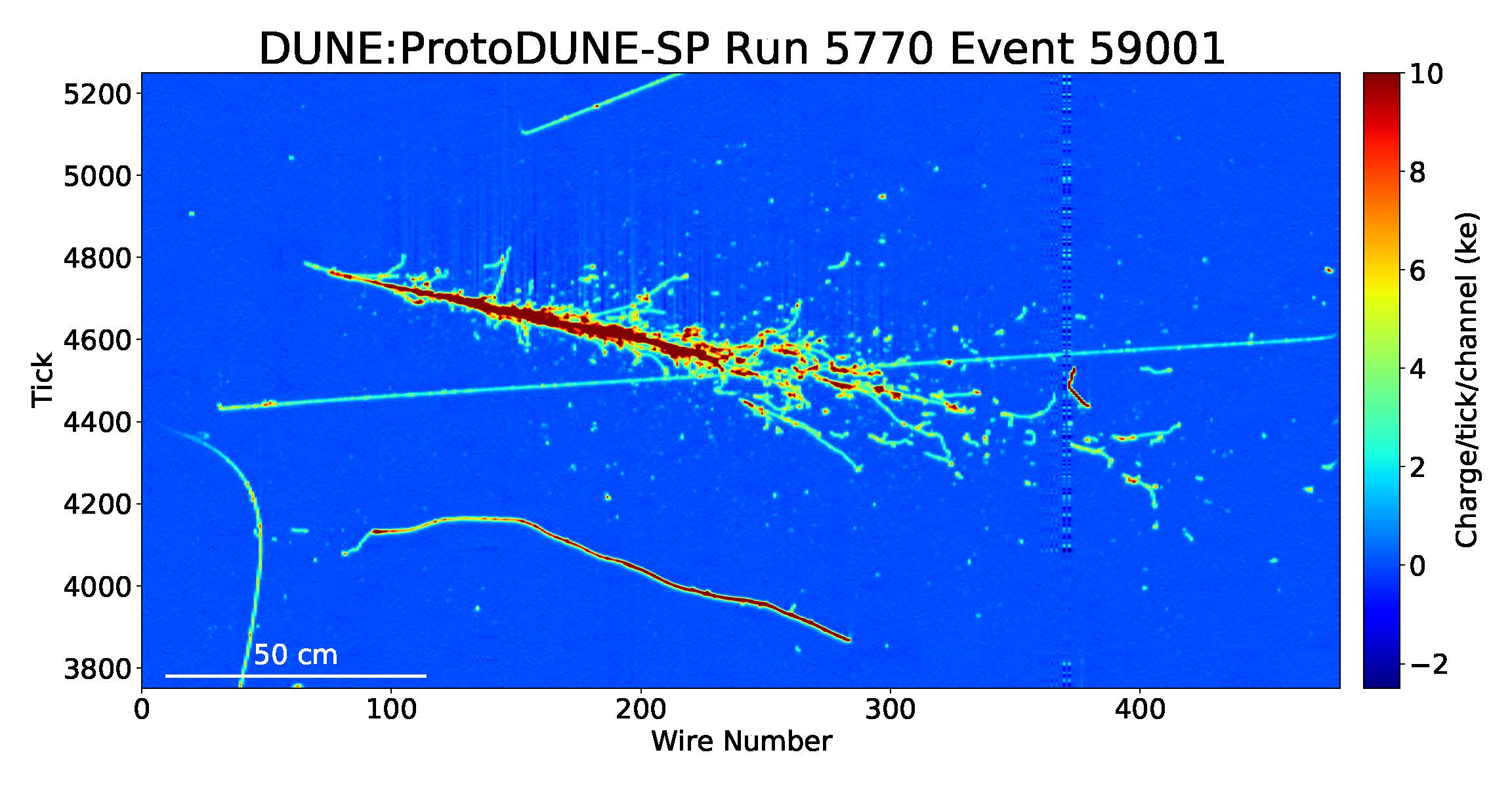
The full offline reconstruction chain for the ProtoDUNE-SP detector is a good representative of event reconstruction in present and future accelerator-based neutrino experiments. For more information, see GPU-accelerated machine learning inference as a service for computing in neutrino experiments.

In each event, charged particles interact with the liquid argon in the detector, liberating ionization electrons that drift across the detector volume under the influence of an electric field.  These electrons induce signals as they pass through and are collected by a set of wire planes at the end of the drift path. Two spatial coordinates can be determined from the different angular orientations of the wires in each plane. The third coordinate can be determined from the drift time of the ionization electrons. As a result, a detailed 3D image of the neutrino interaction can be reconstructed.

The most computationally intensive step of the reconstruction process involves an ML algorithm that looks at 48×48 pixel cutouts, or patches. Those patches represent small sections of the full event and the algorithm identifies the particles in them. Importantly, over the entire ProtoDUNE-SP detector, there are thousands of 48×48 patches to be classified, such that a typical event may have approximately 55,000 patches to process. In the following section, we discuss the performance implications of this process and how using NVIDIA Triton Inference Server helps us to scale the deep learning inference.

Similarly, for the LHC, a series of neural networks can be used to process data from low-level cluster calibration and electron energy regression to jet (particle spray) classification.

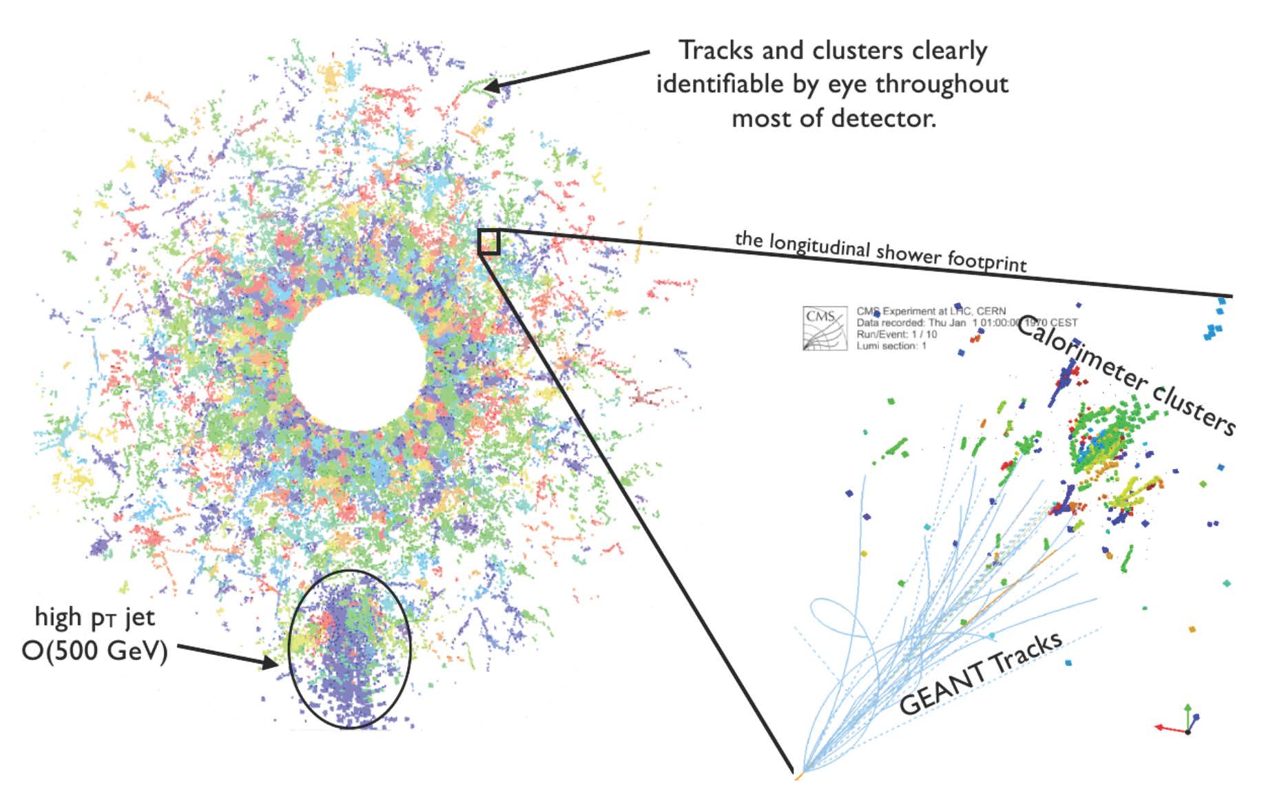
Figure 3 shows how a similar paradigm is used for the LHC. Hits recorded by the calorimeter system are combined into clusters (zoomed-in section at right). These can then be further combined into higher-level reconstructed particle objects, such as the jet indicated at the bottom left. In simulated events such as this one, the reconstructed clusters can be related to the “truth” information from the simulation software (GEANT) to measure the accuracy of the algorithms.

Compute-intensive process

For the ProtoDUNE-SP detector, the reconstruction processing time is dominated by running convolutional neural network inference for the thousands of patches in each event. When you’re running inference on a typical CPU, this consumes 65% of the total time for reconstruction. The current dataset consists of 400 TB from hundreds of millions of neutrino events. The team decided to use NVIDIA T4 GPUs to speed up this most compute-intensive process. In the initial trial phase, they used T4 instances on Google Cloud.

In production, thousands of client nodes feed detector data (images) into the reconstruction process. The scale of computing is so large that a distributed worldwide grid of computing resources is needed. This poses challenges to coordinating and optimizing resources shared by different sites worldwide. To cope with these challenges, the team decided to use a novel inference-as-a-service computing paradigm for the first time.

Inference as a service with NVIDIA Triton Inference Server

The team implemented their generic approach, called SONIC (Services for Optimized Network Inference on Coprocessors), for inference as a service using NVIDIA Triton Inference Server. This technology is available from the NGC Catalog, a hub for GPU-optimized AI containers, models, and SDKs built to simplify and accelerate AI workflows.

NVIDIA Triton simplifies the deployment of AI models at scale in production. It’s an open-source inference serving software package that helps teams deploy trained AI models:

• From any framework: TensorFlow, TensorRT, PyTorch, ONNX Runtime, or a custom framework
• From any storage: Local, Google Cloud Platform, Amazon S3, or Microsoft Azure Storage
• On any GPU- or CPU-based infrastructure: Cloud, data center, or edge

The team deployed the NVIDIA Triton server as a container and used Kubernetes to orchestrate the various cloud resources. Each GPU server in the cluster runs an instance of the NVIDIA Triton server. The clients run on separate, CPU-only nodes and send inference requests using gRPC over the network. Kubernetes handles load balancing and resource scaling for the GPU cluster.

Outcome

The use of T4 GPUs resulted in a 17x speed-up of the most time-consuming ML module of the workflow: track and particle shower hit identification. Overall workflow (event processing time) was accelerated by a factor of 2.7x.

The following are key benefits that the team achieved:

• No disruption. The workflow was accelerated without disruption to any of the other algorithms or experiment software.
• Allocation flexibility. In this deployment, many client nodes sent requests to a single GPU. This allowed heterogeneous resources to be allocated and reallocated based on demand and task, providing significant flexibility and potential cost reduction.
• Reduced dependencies. There’s a reduced dependency on open-source ML frameworks in the experimental code base. Otherwise, the experiment would be required to integrate and support separate C++ APIs for every framework in use.
• Concurrent use. NVIDIA Triton also used all available GPUs automatically when the servers had multiple GPUs, further increasing the flexibility of the server. In addition, NVIDIA Triton can execute multiple models from various ML frameworks concurrently.
• Dynamic batching. NVIDIA Triton provides dynamic batching, which combines multiple requests into optimally sized batches to perform inference as efficiently as possible for the task at hand. This effectively enables simultaneous processing of multiple events without any changes to the experiment software framework.

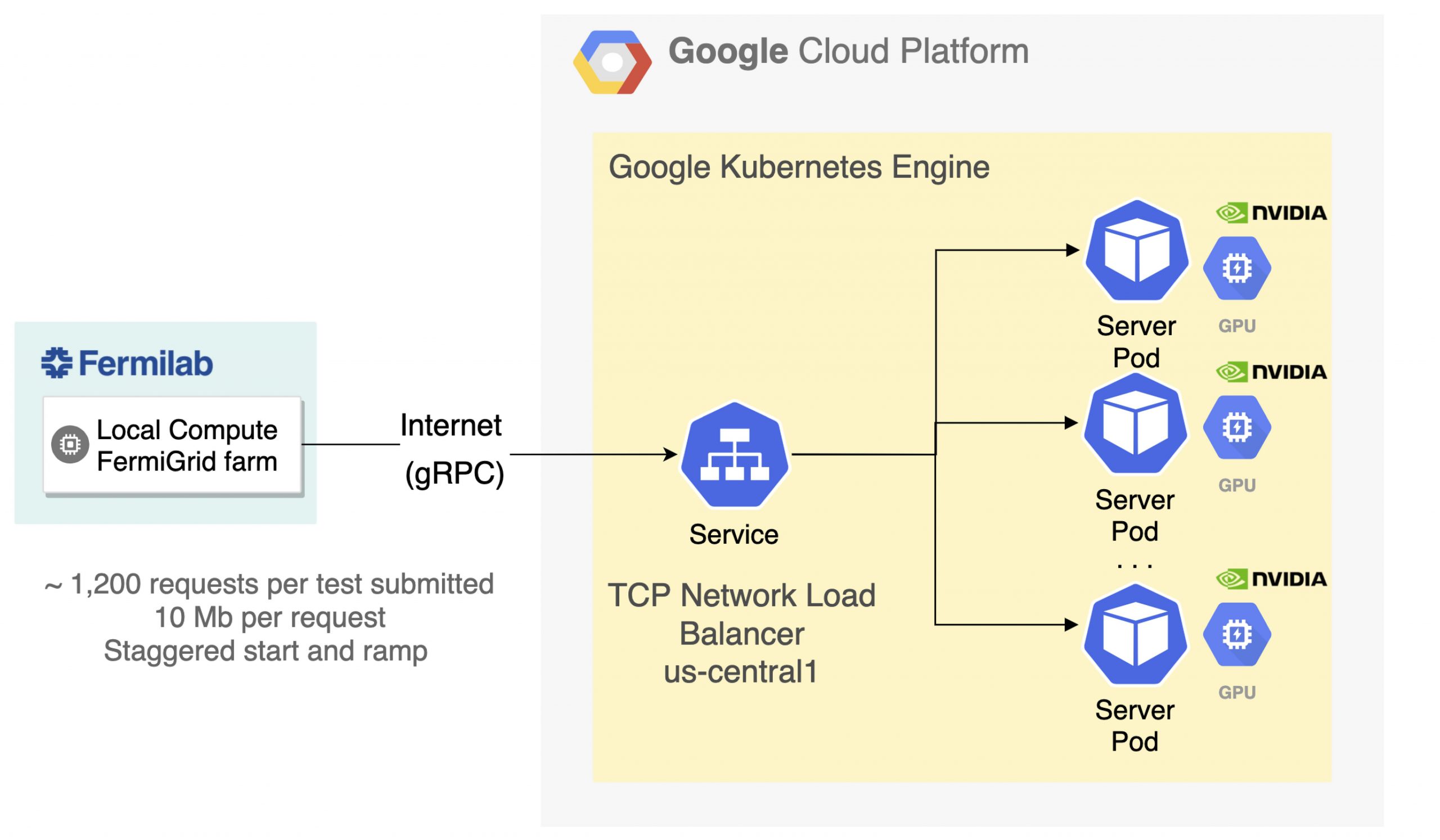
To scale the NVIDIA T4 GPU throughput flexibly, we used a Google Kubernetes Engine (GKE) cluster for server-side workloads. Kubernetes Ingress was used as a load-balancing service to distribute incoming network traffic among the NVIDIA Triton pods. Prometheus-based monitoring was used for the following:

• System metrics from the underlying virtual machine
• Kubernetes metrics for the overall health and state of the cluster
• Inference-specific metrics gathered from NVIDIA Triton through a built-in Prometheus publisher

All metrics were visualized through a Grafana instance, also deployed within the same cluster. The team kept the pod-to-node ratio at 1:1 throughout the studies, with each pod running an instance of NVIDIA Triton Inference Server (v20.02-py3) from NGC. The throughput was maximized when 68 CPU client processes sent requests to a single remote GPU. The exact ratio depends on the algorithm and workflow.

Summary

The offline neutrino reconstruction workflow was accelerated by deploying ML models on NVIDIA T4 GPUs. NVIDIA Triton and Kubernetes helped the team implement inference as a scalable service in a flexible and cost-effective way. Though we focused on a result specific to neutrino physics, a similar result was achieved for the LHC and constitutes a successful proof of concept. These results pave the way for deploying DL inference as a service at scale in high energy physics experiments.

For more information, see the following resources:

• Neutrino (ProtoDUNE) results
• LHC (CMS/ATLAS) results
• SONIC approach
• NVIDIA Triton Inference Server
• NGC Catalog

Acknowledgments

We would like to thank, globally, the multi-institutional team that performed these neutrino and LHC studies. For more information about their work, see fastmachinelearning.org. Featured image of Protodune detector taken by Maximilien Brice from CERN.

Switzerland-based Assaia International AG is deploying a deep learning solution at Cincinnati/Northern Kentucky International Airport (CVG) to help airport employees monitor the turnaround time between flights.

Switzerland-based Assaia International AG, an NVIDIA Metropolis partner and member of the NVIDIA Inception acceleration platform for AI startups, is deploying a deep learning solution at Cincinnati/Northern Kentucky International Airport (CVG) to help airport employees monitor the turnaround time between flights. 

The Turnaround Control tool will help the airport work with its airline partners to improve turnaround transparency, identify situations that most often cause delayed flights, and notify employees of deviations from the schedule. 

“Assaia’s technology adds critical data points to CVG’s early-stage neural network for operational advancements,” said Brian Cobb, the airport’s chief innovation officer. “Structured data generated by artificial intelligence will provide information to make decisions, optimize airside processes, and improve efficiency and safety.”

The company uses NVIDIA Jetson AGX Xavier modules and the NVIDIA Metropolis intelligent video analytics platform to run image recognition and predictive analysis algorithms on video streams from multiple cameras around an airport. 

By installing cameras at several gates, airports can optimize the cleaning, restocking and servicing of planes — saving time for customers and costs for the airlines.

Assaia is also deploying AI solutions at London Gatwick Airport and Seattle-Tacoma International Airport. Watch a replay from the recent GPU Technology Conference for more:

Read more >>

You may have used AI in your smartphone or smart speaker, but have you seen how it comes alive in an artist’s brush stroke, how it animates artificial limbs or assists astronauts in Earth’s orbit? The latest video in the “I Am AI” series — the annual scene setter for the keynote at NVIDIA’s GTC Read article >

The post Around the World in AI Ways: Video Explores Machine Learning’s Global Impact appeared first on The Official NVIDIA Blog.

Today, NVIDIA is announcing the availability of nvCOMP version 2.0.0. This software can be downloaded now free for members of the NVIDIA Developer Program.

Today, NVIDIA is announcing the availability of nvCOMP version 2.0.0. This software can be downloaded now free for members of the NVIDIA Developer Program.

Download Now

What’s New

• Low-level light-weight C interface for expert users featuring batch compression/decompression support and fully asynchronous execution. 
• High-level C/C++ interfaces for ease of use.
• Remove old interfaces.
• Added support for Snappy, Bitcomp, and GDeflate compressors

See the nvCOMP Release Notes for more information

About nvCOMP

nvCOMP is a CUDA library that features generic compression interfaces to enable developers to use high-performance GPU compressors in their applications.

nvCOMP 2.0.0 includes Cascaded, LZ4, and Snappy compression methods. It also adds support for the external Bitcomp and GDeflate methods. Cascaded compression methods demonstrate high performance with up to 500 GB/s throughput and a high compression ratio of up to 80x on numerical data from analytical workloads. Snappy and LZ4 methods can achieve up to 100 GB/s compression and decompression throughput depending on the dataset, and show good compression ratios for arbitrary byte streams.

Learn more:

• GTC 2021: S32401 Optimizing Lossless Compression Algorithms on the GPU
• GTC 2021: CWES1174 Lossless Compression on the GPU
• nvCOMP Project Documentation

Recent Developer Blog posts:

Optimizing Data Transfer Using Lossless Compression with NVIDIA nvcomp

NVIDIA AI Platform Smashes Every MLPerf Category, from Data Center to EdgeSANTA CLARA, Calif., April 21, 2021 (GLOBE NEWSWIRE) — NVIDIA today announced that its AI inference platform, newly …