Google release SpaghettiNet a few months ago. Why did they decide to use a deprecated API for their flagship phone?
https://ai.googleblog.com/2021/11/improved-on-device-ml-on-pixel-6-with.html
submitted by /u/Curld
[visit reddit] [comments]
 DataBloom
Google release SpaghettiNet a few months ago. Why did they decide to use a deprecated API for their flagship phone?
https://ai.googleblog.com/2021/11/improved-on-device-ml-on-pixel-6-with.html
submitted by /u/Curld
[visit reddit] [comments]
So I have a DDQN model, that looks like this:
class DDQN(keras.Model):
def __init__(self, n_actions, fc1_dims, fc2_dims):
super(DDQN, self).__init__()
self.dense1 = keras.layers.Dense(fc1_dims, activation=’relu’)
self.dense1.trainable = True
self.dense2 = keras.layers.Dense(fc2_dims, activation=’relu’)
self.dense1.trainable = True
self.V = keras.layers.Dense(1, activation=None) #Value stream layer
self.V.trainable = True
self.A = keras.layers.Dense(n_actions, activation=None) #Advantage stream layer
self.A.trainable = True
def call(self, state):
x = self.dense1(state)
x = self.dense2(x)
V = self.V(x)
A = self.A(x)
Q = (V + (A – tf.math.reduce_mean(A, axis=1, keepdims=True)))
return Q
def advantage(self, state):
x = self.dense1(state)
x = self.dense2(x)
A = self.A(x)
return A
I do call my model like this:
self.q_eval = DDQN(n_actions, fc1_dims, fc2_dims)
with tf.device(device):
self.q_eval.compile(optimizer=Adam(learning_rate=lr), loss=’mean_squared_error’)
now training and all works, results are great n stuff.
But that’s all pointless, if I can’t save the model, right?
Well, that’s where the trouble began.
def save_model(self):
self.q_eval.save(‘test’)
whenever I call this, I get this error:
Exception has occurred: ValueError
Model <__main__.DDQN object at 0x0000014483B8E948> cannot be saved because the input shapes have not been set. Usually, input shapes are automatically determined from calling `.fit()` or `.predict()`. To manually set the shapes, call `model.build(input_shape)`.
If I do model.build() n shit before saving, nothing changes. Now what would be the proper way to save a model like this?
Please excuse spelling mistakes or dumb sentences in the post and comments, since English is not my native language.
submitted by /u/Chris-hsr
[visit reddit] [comments]
submitted by /u/-is-it-tho
[visit reddit] [comments]
I am new to machine learning.
I got the intermediate result of layer 31 of my CNN using the following code:
conv2d = Model(inputs = self.model_ori.input, outputs= self.model_ori.layers[31].output) intermediateResult = conv2d.predict(img)
Lets say I have this output saved, but 10 days later, I want to take this output and feed it back into the next layer (32nd) and get the final result.
Is that possible?
My model.summary():
submitted by /u/lulzintosh123
[visit reddit] [comments]
I’m very new to tensorflow and machine learning in general and wanted to make something that would take an image of an article of clothing and classify it and remove the background around it. I found a dataset called fashion-MNIST that looks like it might help me with classifying images.
Would it be possible to also use this dataset to get just the pixels of the clothing and remove any background around it? How would I go about doing it and are there any examples that would be helpful for me?
submitted by /u/razz-daddy
[visit reddit] [comments]
Hi,
I am new at using tensorflow-probability. I am using Categorical Distribution to sample a value and then get its probabilty and entropy but every time I sample from the distribution, I get the same entropy. This problem is of policy gradient algorithms. NN outputs logits which are then fed to Categorical distribution then action is sampled. Please let me know, what I am missing here.
submitted by /u/Better-Ad8608
[visit reddit] [comments]
Hello everybody, I’ve run into an error using tensorflow-gpu version 2.7.0. and I am looking for help. Whenever I try to use tensorflow.keras.layers LSTM the kernel of my Jupiter Notebook dies when trying to run model.fit(). I can compile the model and the cell gets executed without an error. I’ve gotten an error message only once and it said:
NotImplementedError: Cannot convert a symbolic Tensor (lstm/strided_slice:0) to a bumpy array. This error may indicate that you’re trying to pass a Tensor to a Num Py call, which is not supported
I’ve only ever gotten this error message once and never again since. I looked it up online and people said it was a compatibility issue with numpy > 1.19.5 so I downgraded numpy but my kernel still dies when trying to do model.fit(). I then tried to pass my training data as a tf tensor by converting the numpy array using tf.convert_to_tensor(). But that didn’t help either. Everything else using tf seems to work, it’s just LSTM giving me issues.
Has anyone an idea how I could fix the issue? Thank you.
Version in use: tensorflow-gpu 2.7.0, Num Py 1.20.3/1.19.5, Cuda 11.3.1 and cudnn 8.1.0.77; GPU: RTX 3090
submitted by /u/0stkreutz
[visit reddit] [comments]
 Introducing the NVIDIA HGX H100, a key GPU server building block powered by the Hopper architecture.
The NVIDIA mission is to accelerate the work of the Da Vincis and Einsteins of our time and empower them to solve the grand challenges of society. With the complexity of artificial intelligence (AI), high-performance computing (HPC), and data analytics increasing exponentially, scientists need an advanced computing platform that is able to drive million-X speedups in a single decade to solve these extraordinary challenges.
To answer this need, we introduce the NVIDIA HGX H100, a key GPU server building block powered by the NVIDIA Hopper Architecture. This state-of-the-art platform securely delivers high performance with low latency, and integrates a full stack of capabilities from networking to compute at data center scale, the new unit of computing.
In this post, I discuss how the NVIDIA HGX H100 is helping deliver the next massive leap in our accelerated compute data center platform.
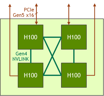
The HGX H100 8-GPU represents the key building block of the new Hopper generation GPU server. It hosts eight H100 Tensor Core GPUs and four third-generation NVSwitch. Each H100 GPU has multiple fourth generation NVLink ports and connects to all four NVSwitches. Each NVSwitch is a fully non-blocking switch that fully connects all eight H100 Tensor Core GPU.
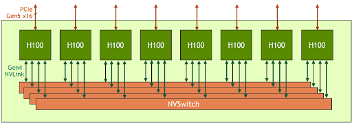
This fully connected topology from NVSwitch enables any H100 to talk to any other H100 concurrently. Notably, this communication runs at the NVLink bidirectional speed of 900 gigabytes per second (GB/s), which is more than 14x the bandwidth of the current PCIe Gen4 x16 bus.
The third-generation NVSwitch also provides new hardware acceleration for collective operations with multicast and NVIDIA SHARP in-network reductions. Combining with the faster NVLink speed, the effective bandwidth for common AI collective operations like all-reduce go up by 3x compared to the HGX A100. The NVSwitch acceleration of collectives also significantly reduces the load on the GPU.
| HGX A100 8-GPU | HGX H100 8-GPU | Improvement Ratio | |
| FP8 | – | 32,000 TFLOPS | 6X (vs A100 FP16) |
| FP16 | 4,992 TFLOPS | 16,000 TFLOPS | 3X |
| FP64 | 156 TFLOPS | 480 TFLOPS | 3X |
| In-Network Compute | 0 | 3.6 TFLOPS | Infinite |
| Interface to host CPU | 8x PCIe Gen4 x16 | 8x PCIe Gen5 x16 | 2X |
| Bisection Bandwidth | 2.4 TB/s | 3.6 TB/s | 1.5X |
*Note: FP performance includes sparsity
The emerging class of exascale HPC and trillion parameter AI models for tasks like accurate conversational AI require months to train, even on supercomputers. Compressing this to the speed of business and completing training within hours requires high-speed, seamless communication between every GPU in a server cluster.
To tackle these large use cases, the new NVLink and NVSwitch are designed to enable HGX H100 8-GPU to scale up and support a much larger NVLink domain with the new NVLink-Network. Another version of HGX H100 8-GPU features this new NVLink-Network support.
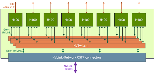
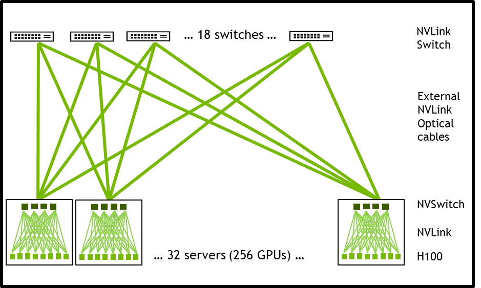
System nodes built with HGX H100 8-GPU with NVLink-Network support can fully connect to other systems through the Octal Small Form Factor Pluggable (OSFP) LinkX cables and the new external NVLink Switch. This connection enables up to a maximum of 256 GPU NVLink domains. Figure 3 shows the cluster topology.
| 256 A100 GPU Pod | 256 H100 GPU Pod | Improvement Ratio | |
| NVLINK Domain | 8 GPU | 256 GPU | 32X |
| FP8 | – | 1,024 PFLOPS | 6X (vs A100 FP16) |
| FP16 | 160 PFLOPS | 512 PFLOPS | 3X |
| FP64 | 5 PFLOPS | 15 PFLOPS | 3X |
| In-Network Compute | 0 | 192 TFLOPS | Infinite |
| Bisection Bandwidth | 6.4 TB/s | 70 TB/s | 11X |
*Note: FP performance includes sparsity
With the dramatic increase in HGX H100 compute and networking capabilities, AI and HPC applications performances are vastly improved.
Today’s mainstream AI and HPC model can fully reside in the aggregate GPU memory of a single node. For example, BERT-Large, Mask R-CNN, and HGX H100 are the most performance-efficient training solutions.
For the more advanced and larger AI and HPC model, the model requires multiple nodes of aggregate GPU memory to fit. For example, a deep learning recommendation model (DLRM) with terabytes of embedded tables, a large mixture-of-experts (MoE) natural language processing model, and the HGX H100 with NVLink-Network accelerates the key communication bottleneck and is the best solution for this class of workload.
Figure 4 from the NVIDIA H100 GPU Architecture whitepaper shows the extra performance boost enabled by the NVLink-Network.
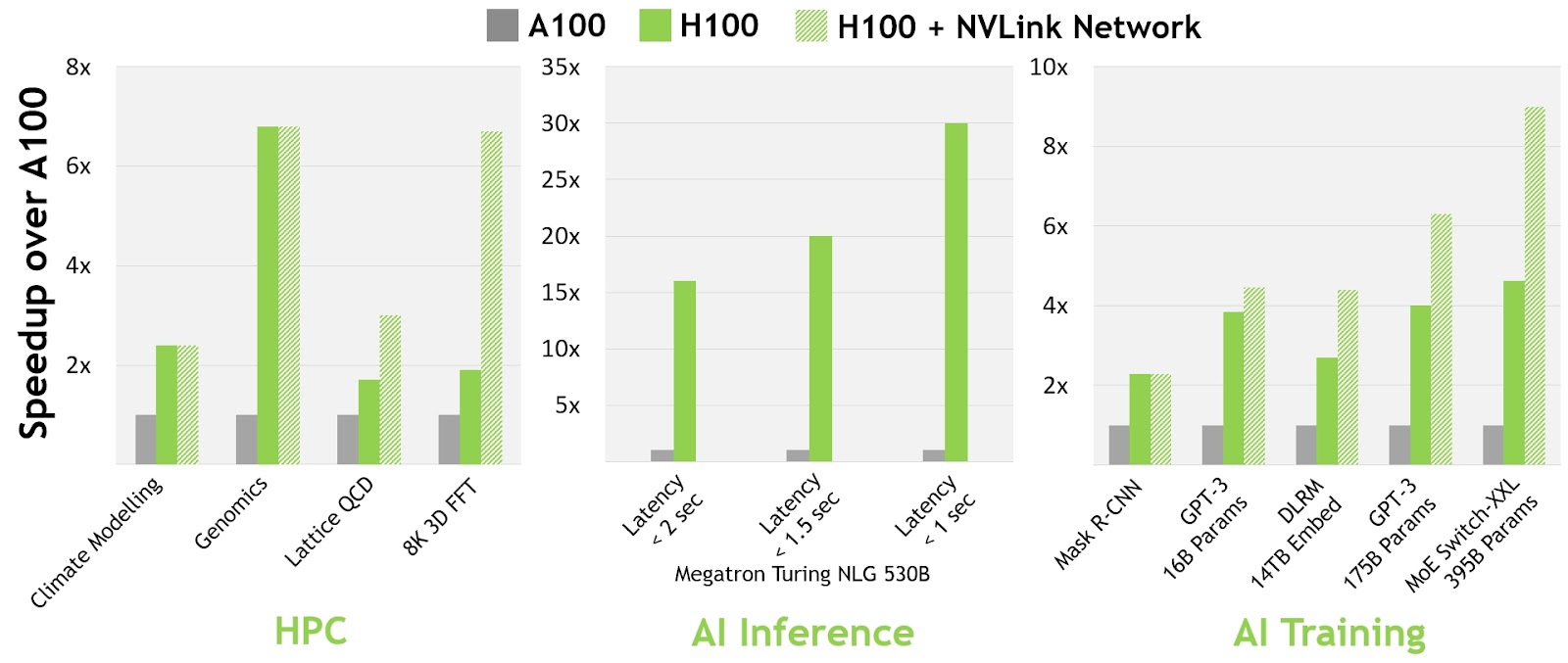
All performance numbers are preliminary based on current expectations and subject to change in shipping products. A100 cluster: HDR IB network. H100 cluster: NDR IB network with NVLink-Network where indicated.
# GPUs: Climate Modeling 1K, LQCD 1K, Genomics 8, 3D-FFT 256, MT-NLG 32 (batch sizes: 4 for A100, 60 for H100 at 1 sec, 8 for A100 and 64 for H100 at 1.5 and 2sec), MRCNN 8 (batch 32), GPT-3 16B 512 (batch 256), DLRM 128 (batch 64K), GPT-3 16K (batch 512), MoE 8K (batch 512, one expert per GPU)
In addition to the 8-GPU version, the HGX family also features a version with a 4-GPU, which is directly connected with fourth-generation NVLink.
The H100-to-H100 point-to-point peer NVLink bandwidth is 300 GB/s bidirectional, which is about 5X faster than today’s PCIe Gen4 x16 bus.
The HGX H100 4-GPU form factor is optimized for dense HPC deployment:
NVIDIA is working closely with our ecosystem to bring the HGX H100 based server platform to the market later this year. We are looking forward to putting this powerful computing tool in your hands, enabling you to innovate and fulfill your life’s work at the fastest pace in human history.
 cuTENSOR is now able to distribute tensor contractions across multiple GPUs. This has been released as a new library called cuTENSORMg (multi-GPU).
Tensor contractions are at the core of many important workloads in machine learning, computational chemistry, and quantum computing. As scientists and engineers pursue ever-growing problems, the underlying data gets larger in size and calculations take longer and longer.
When a tensor contraction does not fit into a single GPU anymore, or if it takes too long on a single GPU, the natural next step is to distribute the contraction across multiple GPUs. We have been extending cuTENSOR with this new capability, and are releasing it as a new library called cuTENSORMg (multi-GPU). It provides single-process multi-GPU functionality on block-cyclic distributed tensors.
The copy and contraction operations for cuTENSORMg are broadly structured into handles, tensor descriptors, and descriptors. In this post, we explain the handle and the tensor descriptor and how copy operations work and demonstrate how to perform a tensor contraction. We then show how to measure the performance of the contraction operation for various workloads and GPU configurations.
The library handle represents the set of devices that participate in the computation. The handle also contains data and resources that are reused across calls. You can create a library handle by passing the list of devices to the cutensorMgCreate function:
cutensorMgCreate(&handle, numDevices, devices);
All objects in cuTENSORMg are heap allocated. As such, they must be freed with a matching destroy call. For brevity, we do not show these in this post, but production code should destroy all objects that it creates to avoid leaks.
cutensorMgDestroy(handle);All library calls return an error code of type cutensorStatus_t. In production, you should always check the error code to detect failures or usage issues early. For brevity, we omit these checks in this post for brevity, but they are included in the corresponding example code.
In addition to error codes, cuTENSORMg also provides similar logging capabilities as cuTENSOR. Those logs can be activated by setting the CUTENSORMG_LOG_LEVEL environment variable appropriately. For instance, CUTENSORMG_LOG_LEVEL=1 would provide you with additional information about a returned error code.
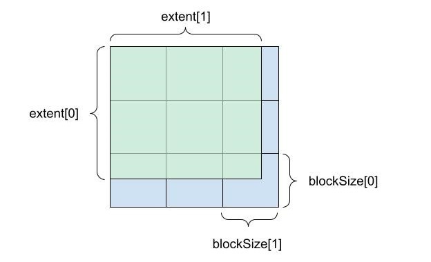
The tensor descriptor describes how a tensor is laid out in memory and how it is distributed across devices. For each mode, there are three core concepts to determine the layout:
extent: Logical size of each mode.blockSize: Subdivides the extent into equal-sized chunks, except for the final remainder block.deviceCount: Determines how the blocks are distributed across devices.Figure 1 shows how extent and block size subdivide a two-dimensional tensor.
![A 3x3 square showing deviceCount [0] on the Y axis and deviceCount[1] on the X axis.](https://developer-blogs.nvidia.com/wp-content/uploads/2022/03/Introducing-Multi-GPU-Tensor-Contractions-4-625x494_2.jpg)
Blocks are distributed in a cyclic fashion, which means that consecutive blocks are assigned to different devices. Figure 2 shows a two-by-two distribution of blocks to devices, with the assignment of devices to blocks being encoded with another array devices. The array is a dense-column major tensor with extents like the device counts.
![A 4x4 block with Y axis as blockStride[0] and X axis blockStride[1]. This block is comprised of smaller by 4x4 blocks with elementStride[1] as the X axis and and elementStride[0] as the Y axis.](https://developer-blogs.nvidia.com/wp-content/uploads/2022/03/Introducing-Multi-GPU-Tensor-Contractions-2-625x469_2.jpg)
Finally, the exact on-device data layout is determined by the elementStride and the blockStride values for each mode. Respectively, they determine the displacement, in linear memory in units of elements, of two adjacent elements and adjacent blocks for a given mode (Figure 3).
These attributes are all set using the cutensorMgCreateTensorDescriptor call:
cutensorMgCreateTensorDescriptor(handle, &desc, numModes, extent, elementStride, blockSize, blockStride, deviceCount, numDevices, devices, type);
It is possible to pass NULL to the elementStride, blockSize, blockStride, and deviceCount.
If the elementStride is NULL, the data layout is assumed to be dense using a generalized column-major layout. If blockSize is NULL, it is equal to extent. If blockStride is NULL, it is equal to blockSize * elementStride, which results in an interleaved block format. If deviceCount is NULL, all device counts are set to 1. In this case, the tensor is distributed and entirely resides in the memory of devices[0].
By passing CUTENSOR_MG_DEVICE_HOST as the owning device, you can specify that the tensor is located on the host in pinned, managed, or regularly allocated memory.
The copy operation enables data layout changes including the redistribution of the tensor to different devices. Its parameters are a source and a destination tensor descriptor (descSrc and descDst), as well as a source and destination mode list (modesSrc and modesDst). The two tensors’ extents at coinciding modes must match, but everything else about them may be different. One may be located on the host, the other across devices, and they may have different blockings and different strides.
Like all operations in cuTENSORMg, it proceeds in three steps:
cutensorMgCopyDescriptor_t: Encodes what operation should be performed.cutensorMgCopyPlan_t: Encodes how the operation will be performed.cutensorMgCopy: Performs the operation according to the plan.The first step is to create the copy descriptor:
cutensorMgCreateCopyDescriptor(handle, &desc, descDst, modesDst, descSrc, modesSrc);With the copy descriptor in hand, you can query the amount of device-side and host-side workspace that is required. The deviceWorkspaceSize array has as many elements as there are devices in the handle. The i-th element is the amount of workspace required for the i-th device in the handle.
cutensorMgCopyGetWorkspace(handle, desc, deviceWorkspaceSize, &hostWorkspaceSize);
With the workspace sizes determined, plan the copy. You can pass a larger workspace size and the call may take advantage of more workspace, or you can try to pass a smaller size. The planning may be able to accommodate that or it may yield an error.
cutensorMgCreateCopyPlan(handle, &plan, desc, deviceWorkspaceSize, hostWorkspaceSizeFinally, with the planning complete, execute the copy operation.
cutensorMgCopy(handle, plan, ptrDst, ptrSrc, deviceWorkspace, hostWorkspace, streams);In this call, ptrDst and ptrSrc are arrays of pointers. They contain one pointer for each of the devices in the corresponding tensor descriptor. In this instance, ptrDst[0] corresponds to the device that was passed as devices[0] to cutensorMgCreateTensorDescriptor.
On the other hand, deviceWorkspace and streams are also arrays where each entry corresponds to a device. They are ordered according to the order of devices in the library handle, such as deviceWorkspace[0] and streams[0] correspond to the device that was passed at devices[0] to cutensorMgCreate. The workspaces must be at least as large as the workspace sizes that were passed to cutensorMgCreateCopyPlan.
At the core of the cuTENSORMg library is the contraction operation. It currently implements tensor contractions of tensors located on one or multiple devices, but may support tensors located on the host in the future. As a refresher, a contraction is an operation of the following form:
Where 


Like the copy operation, it proceeds in three stages:
cutensorMgCreateContractionDescriptor: Encodes the problem.cutensorMgCreateContractionPlan: Encodes the implementation.cutensorMgContraction: Uses the plan and performs the actual contraction.First, you create a contraction descriptor based on the tensor descriptors, mode lists, and the desired compute type, such as the lowest precision data that may be used during the calculation.
cutensorMgCreateContractionDescriptor(handle, &desc, descA, modesA, descB, modesB, descC, modesC, descD, modesD, compute);
As the contraction operation has more degrees of freedom, you must also initialize a find object that gives you finer control over the plan creation for a given problem descriptor. For now, this find object only has a default setting:
cutensorMgCreateContractionFind(handle, &find, CUTENSORMG_ALGO_DEFAULT);
Then, you can query the workspace requirement along the lines of what you did for the copy operation. Compared to that operation, you also pass in the find and a workspace preference:
cutensorMgContractionGetWorkspace(handle, desc, find, CUTENSOR_WORKSPACE_RECOMMENDED, deviceWorkspaceSize, &hostWorkspaceSize);
Create a plan:
cutensorMgCreateContractionPlan(handle, &plan, desc, find, deviceWorkspaceSize, hostWorkspaceSize);
Finally, execute the contraction using the plan:
cutensorMgContraction(handle, plan, alpha, ptrA, ptrB, beta, ptrC, ptrD, deviceWorkspace, hostWorkspace, streams);
In this call, alpha and beta are host pointers of the same type as the BFloat16 precision, in which case it is single precision. The order of pointers in the different arrays ptrA, ptrB, ptrC, and ptrD correspond to their order in their descriptor’s devices array. The order of pointers in the deviceWorkspace and streams arrays corresponds to the order in the library handle’s devices array.
You can find all these calls together in the CUDA Library Samples GitHub repo. We extended it to take two parameters: The number of GPUs and a scaling factor. Feel free to experiment with other contractions, block sizes, and scaling regimes. It is written in such a way that it scales up M and N while keeping K fixed. It implements an almost GEMM-shaped tensor contraction of the shape:


Interested in trying out cuTENSORMg to scale tensor contractions beyond a single GPU?
We continue working on improving cuTENSORMg, including out-of-core functionality. If you have questions or new feature requests, contact product manager Matthew Nicely US.
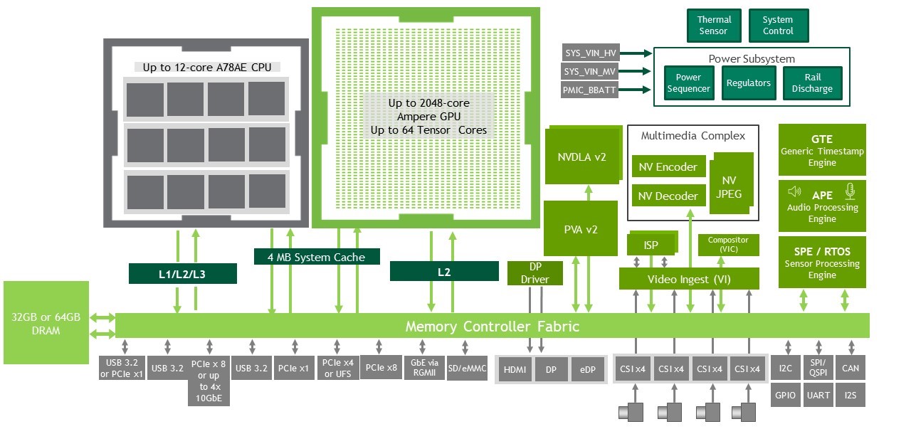
 Get started with developing all four Jetson Orin modules for a new era of robotics.
The pace for development and deployment of AI-powered robots and other autonomous machines continues to grow rapidly. The next generation of applications require large increases in AI compute performance to handle multimodal AI applications running concurrently in real time.
Human-robot interactions are increasing in retail spaces, food delivery, hospitals, warehouses, factory floors, and other commercial applications. These autonomous robots must concurrently perform 3D perception, natural language understanding, path planning, obstacle avoidance, pose estimation, and many more actions that require both significant computational performance and highly accurate trained neural models for each application.
NVIDIA Jetson AGX Orin modules are the highest-performing and newest members of the NVIDIA Jetson family. These modules deliver tremendous performance with class-leading energy efficiency. They run the comprehensive NVIDIA AI software stack to power the next generation of demanding edge AI applications.
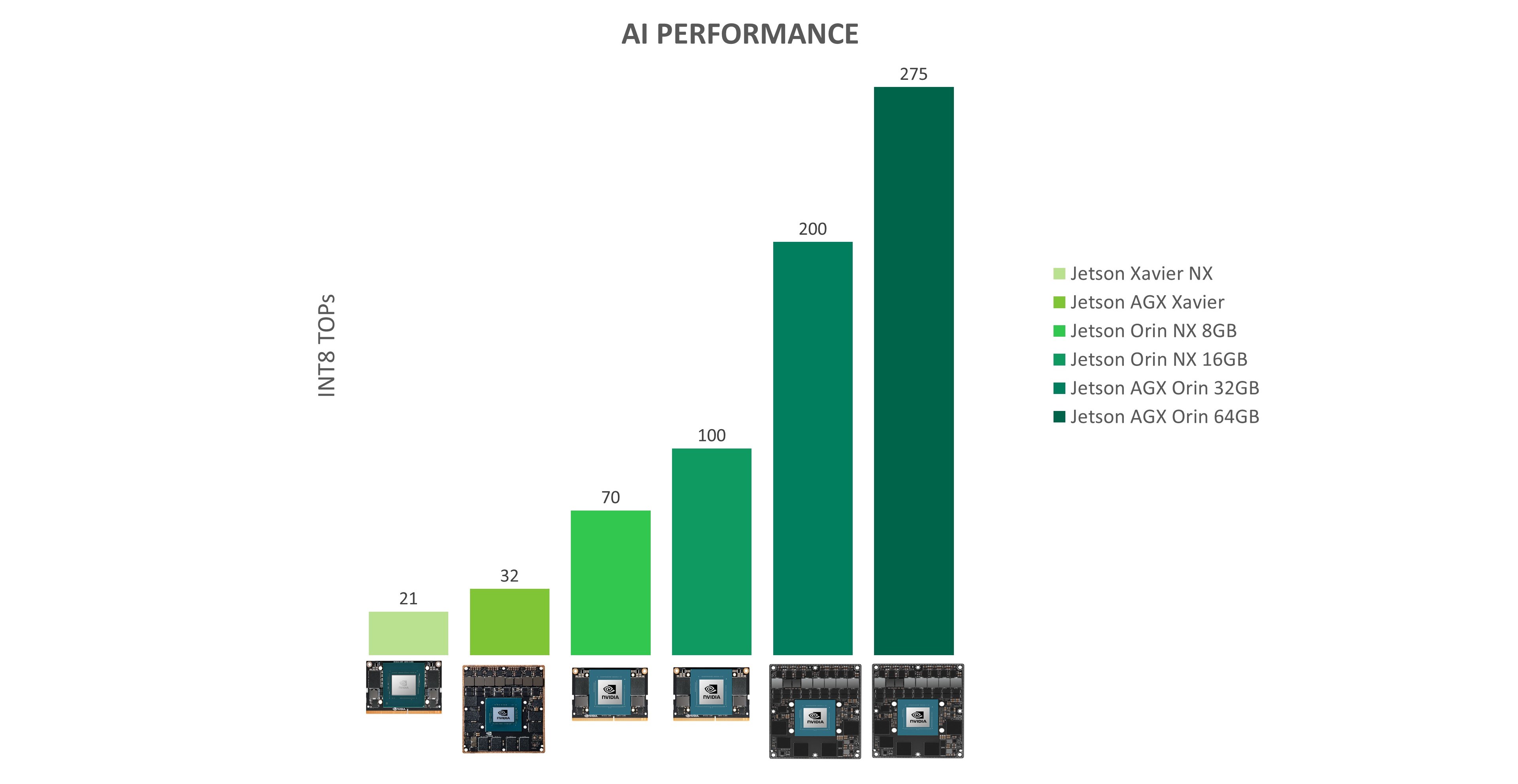
At GTC Spring 2022, we announced that four Jetson Orin modules will be available in Q4 2022. With up to 275 tera operations per second (TOPS) of performance, the Jetson Orin modules can run server class AI models at the edge with end-to-end application pipeline acceleration. Compared to Jetson Xavier modules, Jetson Orin brings even higher performance, power efficiency, and inference capabilities to modern AI applications.
| JETSON AGX XAVIER 64GB | JETSON AGX ORIN 64GB | |
| 21 DENSE INT8 TOPS | 275 SPARSE|138 DENSE, INT8 TOPS | |
| 10W to 20W | 15W to 60W | |
| $499 (1KU+) | $1,599 (1KU+) | |
| JETSON XAVIER NX 8GB | JETSON AGX ORIN 32GB | |
| 32 DENSE INT8 TOPS | 200 SPARSE|100 DENSE, INT8 TOPS | |
| 10W to 30W | 15W to 40W | |
| $899 (1KU+) | $899 (1KU+) | |
| JETSON XAVIER NX 16GB | JETSON ORIN NX 16GB | |
| 21 DENSE INT8 TOPS | 100 SPARSE|50 DENSE, INT8 TOPS | |
| 10W to 20W | 10W to 25W | |
| $499 (1KU+) | $599 (1KU+) | |
| JETSON XAVIER NX 8GB | JETSON ORIN NX 16GB | |
| 21 DENSE INT8 TOPS | 100 SPARSE|50 DENSE, INT8 TOPS | |
| 10W to 20W | 10W to 25W | |
| $399 (1KU+) | $599 (1KU+) |
The Jetson AGX Orin series includes the Jetson AGX Orin 64GB and the Jetson AGX Orin 32GB modules.
These modules have the same compact form factor and are pin compatible with Jetson AGX Xavier series modules, offering you an 8x performance upgrade, or up to 6x the performance at the same price.
Edge and embedded systems continue to be driven by the increasing number, performance, and bandwidth of sensors. The Jetson AGX Orin series brings not only additional compute for processing these sensors, but also additional I/O:
For more information, see the Jetson Orin product page and the Jetson AGX Orin Series Data Sheet.
USB 3.2, UFS, MGBE, and PCIe share UPHY Lanes. For the supported UPHY configurations, see the Design Guide.
The NVIDIA Orin NX series includes Jetson Orin NX 16GB with up to 100 TOPS of AI performance, and Jetson Orin NX 8GB with up to 70 TOPS. With this series, we followed a similar design philosophy as with Jetson Xavier NX. We brought the NVIDIA Orin architecture and brought it to the smallest Jetson form factor, 260-pin SODIMM, with lower power consumption.
You can bring this higher class of performance to your next-generation, small form factor products like drones and handheld devices. Jetson Orin NX 16GB comes with power configurable between 10W and 25W, and Jetson Orin NX 8GB comes with power configurable between 10W and 20W.
The Orin NX Series is form factor compatible with the Jetson Xavier NX series, and delivers up to 5x the performance, or up to 3X the performance at the same price. The Orin NX series also brings additional high speed I/O capabilities with up to seven PCIe lanes and three 10Gbps USB 3.2 interfaces. For storage, you can leverage the additional PCIe lanes to connect to external NVMe. For more information, see the Jetson Orin product page.
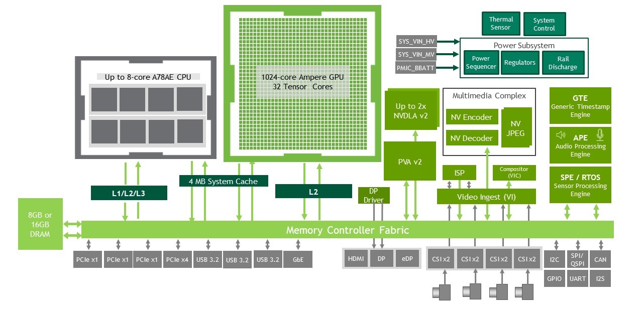
Jetson AGX Xavier was designed around the NVIDIA Xavier SoC, our first architecture developed from the ground up for autonomous machines. The NVIDIA Orin architecture takes this class of product to the next level. It continues to showcase multiple different on-chip processors, but brings greater capability, higher performance, and more power efficiency.
The Jetson Orin modules contain the following:
Like the other Jetson modules, Jetson Orin is built using a system-on-module (SOM) design. All the processing, memory, and power rails are contained on the module. All the high-speed I/O is available through a 699-pin connector (Jetson AGX Orin series) or a 260-pin SODIMM connector (Jetson Orin NX series). This SOM design makes it easy for you to integrate the modules into your system designs.
At GTC 2022, NVIDIA also announced availability of the Jetson AGX Orin Developer Kit. The developer kit contains everything needed for you to get up and running quickly. It includes a Jetson AGX Orin module with the highest performance and runs the world’s most advanced deep learning software stack. This kit delivers the flexibility to create sophisticated AI solutions now and well into the future.
Compact size, high-speed interfaces, and lots of connectors make this developer kit perfect for prototyping advanced AI-powered robots and edge applications for manufacturing, logistics, retail, service, agriculture, smart cities, healthcare, life sciences, and more.
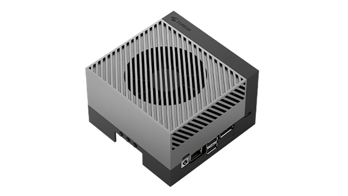
Jetson AGX Orin Developer Kit features:
The Jetson AGX Orin Developer Kit runs the latest NVIDIA JetPack 5.0 software. NVIDIA JetPack 5.0 supports emulating the performance and clock frequencies of Jetson Orin NX and Jetson AGX Orin series modules with a Jetson AGX Orin Developer Kit. You can kickstart your development for any of those modules today.
Jetson AGX Orin Developer Kit is available for purchase through NVIDIA authorized distributors worldwide. Get started today by following the Getting Started guide.
| Developer Kit | AGX Orin 64GB | AGX Orin 32GB | |
| AI Performance | 275 INT8 Sparse TOPs | 200 INT8 Sparse TOPs | |
| GPU | 2048-core NVIDIA Ampere Architecture GPU with 64 Tensor Cores |
1792-core NVIDIA Ampere Architecture GPU with 56 Tensor Cores | |
| CPU | 12-core Arm Cortex-A78AE v8.2 64-bit CPU 3MB L2 + 6MB L3 |
8-core Arm Cortex-A78AE v8.2 64-bit CPU 2MB L2 + 4MB L3 |
|
| Power | 15W-60W | 15W-40W | |
| Memory | 32 GB | 64 GB | 32GB |
| MSRP | $1,999 | $1,599 | $899 |
Table 2. Summary comparison of Jetson AGX Orin series modules and Developer Kit
Jetson Orin provides a giant leap forward for your next generation applications. Using the Jetson AGX Orin Developer Kit, we have taken the geometric mean of measured performance for our highly accurate, production-ready, pretrained models for computer vision and conversational AI. Testing included the following benchmarks:
With the NVIDIA JetPack 5.0 Developer Preview, Jetson AGX Orin shows a 3.3X performance increase compared to Jetson AGX Xavier. With future software improvements, we expect this to approach a 5X performance increase. Jetson AGX Xavier performance has increased 1.5X since NVIDIA JetPack 4.1.1 Developer Preview, the first software release to support it.
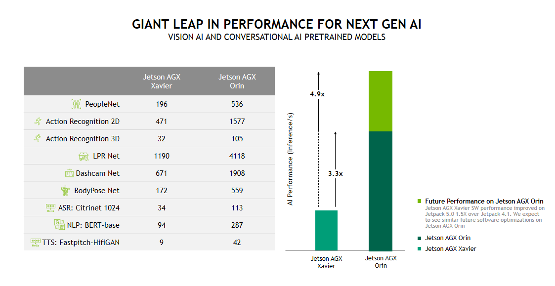
The benchmarks have been run on our Jetson AGX Orin Developer Kit. PeopleNet and DashcamNet provide examples of dense models that can be run concurrently on the GPU and the two DLAs. The DLA can be used to offload some AI applications from the GPU and this concurrent capability enables them to operate in parallel.
PeopleNet, LPRNet, DashcamNet, and BodyPoseNet provide examples of dense INT8 benchmarks run on Jetson. ActionRecognitionNet 2D and 3D and the conversational AI benchmarks provide examples of dense FP16 performance. All these models can be found on NVIDIA NGC.
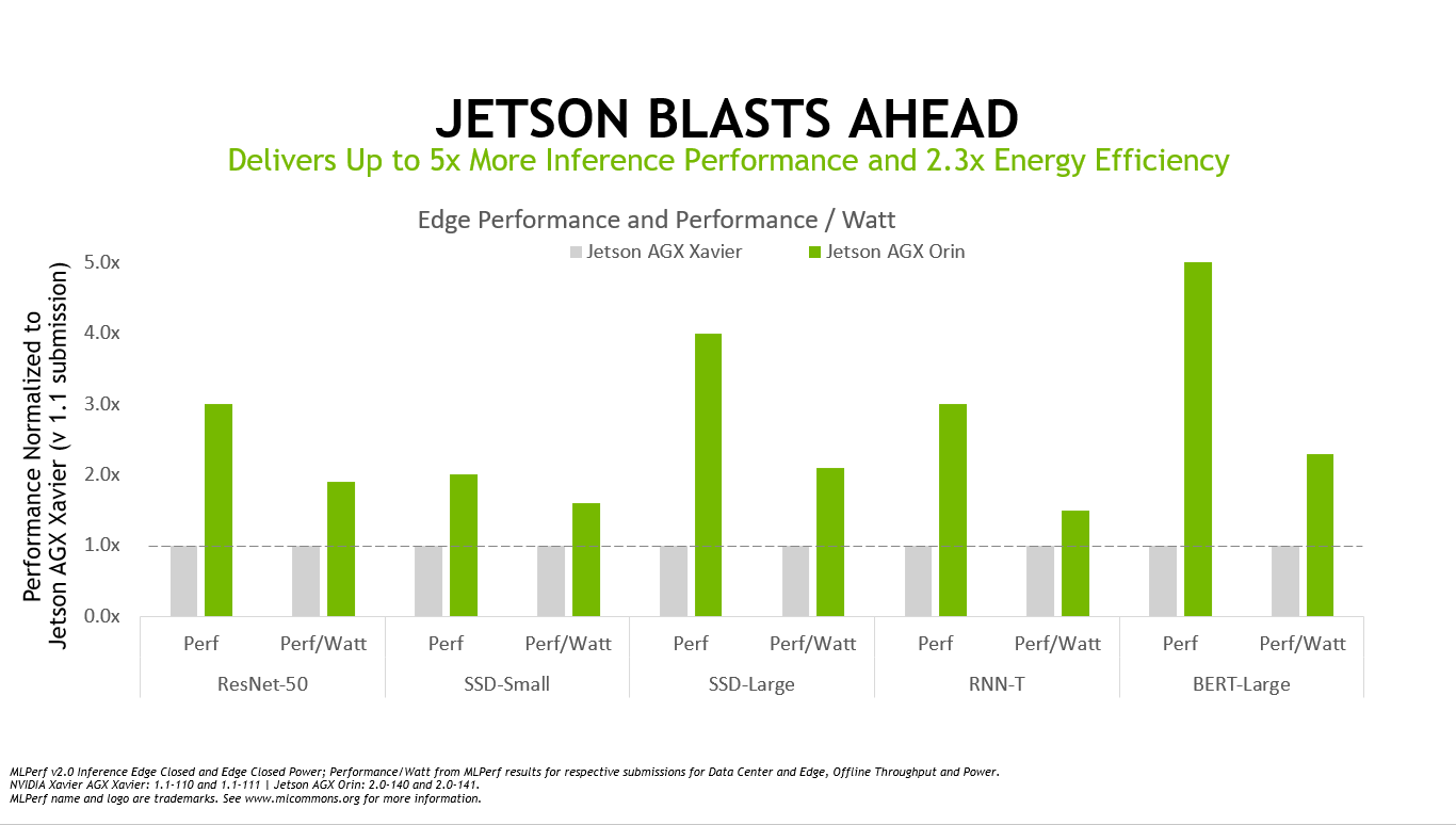
Moreover, Jetson Orin continues to raise the bar for AI at the edge, adding to the NVIDIA overall top rankings in the latest MLPerf industry inference benchmarks. Jetson AGX Orin provides up to a 5X performance increase on these MLPerf benchmarks compared to previous results on Jetson AGX Xavier, while delivering an average of 2x better energy efficiency.
The class-leading performance and energy efficiency of Jetson Orin is backed by the same powerful NVIDIA AI software that is deployed in GPU-accelerated data centers, hyperscale servers, and powerful AI workstations.
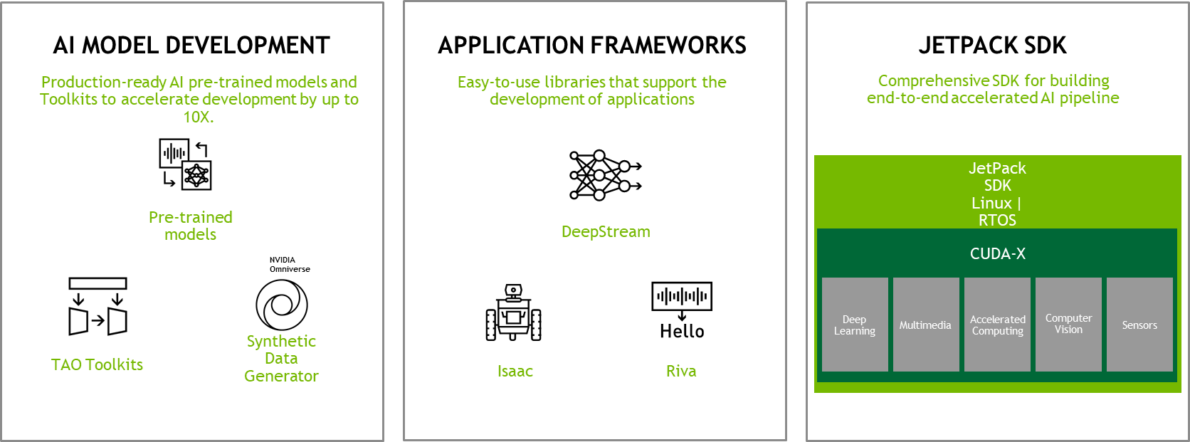
NVIDIA JetPack is the foundational SDK for the Jetson platform. NVIDIA JetPack provides a full development environment for hardware-accelerated AI-at-the-edge development. Jetson Orin is supported by NVIDIA JetPack 5.0, which includes the following:
NVIDIA JetPack 5.0 also supports Jetson Xavier modules.
For you to develop fully accelerated applications quickly on the Jetson platform, NVIDIA provides application frameworks for various use cases:
To accelerate the time to develop production-ready and highly accurate AI models, NVIDIA provides various tools to generate training data, train and optimize models, and quickly create ready to deploy AI models.
The NVIDIA Omniverse Replicator for synthetic data generation helps in creating high-quality datasets to boost model training. With Omniverse Replicator, you can create large and diverse synthetic datasets that is not only hard but sometimes impossible to create in the real world. Using synthetic data along with real data for training the model, you can significantly improve the model accuracy.
NVIDIA pretrained models from NGC start you off with highly accurate and optimized models and model architectures for various use cases. Pretrained models are production-ready. You can further customize these models by training with your own real or synthetic data, using the NVIDIA TAO (Train-Adapt-Optimize) workflow to quickly build an accurate and ready to deploy model.
Watch these NVIDIA technologies coming together on Jetson AGX Orin for a robotic use case.
Learn about everything in the Jetson AGX Orin Developer Kit in this getting started video:
For more information about all the NVIDIA technologies that we bring in NVIDIA Jetson Orin modules, watch a webinar on Jetson software.
Get started with developing all four Jetson Orin modules by placing an order for the Jetson AGX Orin Developer Kit, and downloading the NVIDIA JetPack 5.0 SDK. Additional documentation for Jetson AGX Orin can be found at the download center. For information and support, visit the NVIDIA Embedded Developer page and forums for help from community experts.

