In record time, Vikram Gavini’s lab crossed a big milestone in viewing tiny things. The three-person team at the University of Michigan crafted a program that uses complex math to peer deep into the world of the atom. It could advance many fields of science, as well as the design for everything from lighter cars Read article >
GFN Thursday is all about bringing games powered by GeForce NOW’s GPUs in the cloud to gamers. Today, that spotlight shines on Team17, the prolific publisher behind many games in the GeForce NOW library. The party gets started with their newest release, a day-and-date launch of Sheltered 2, streaming on the cloud alongside the 12 Read article >
So, like the title says. Just wondering if there is anything like this. I know that StackOverflow has stuff like that, but rather ask on slack or something similar.
According to my understanding, the output consists of three (5, 5) matrices stacked together. However, printing ‘out’ shows five (5, 3) matrices stacked together:
Independent IT lab The Tolly Group compared the cloud, AI, and storage performance of an NVIDIA Ethernet switch to the performance of a comparable switch built with commodity silicon.
Does the switch matter?
The network fabric is key to the performance of modern data centers. There are many requirements for data center switches, but the most basic is to provide equal amounts of bandwidth to all clients so that resources are shared evenly. Without fair networking, all workloads experience unpredictable performance due to throughput deterioration, delay, slow distributed workloads, and so on.
To answer the question of whether the switch matters, the Tolly Group benchmarked the cloud, AI, and storage workload performance of the NVIDIA Spectrum-3 12.8Tbps Switch. It compared the results to the performance of a typical (commodity) 12.8 Tbps data center switch, in an apples-to-apples comparison.
The Tolly Group
The Tolly Group, a third-party, independent IT industry lab, has been conducting performance tests and hands-on evaluations of IT products for more than 30 years. The Tolly Group is positioned to provide evidence that products meet or exceed marketing claims and they won’t produce reports that conflict with The Tolly Group’s Fair Testing Charter. This proof-of-performance lets customers know they can deploy with confidence.
Distributed workload performance (AI and SPARK)
Every switch has a buffer to prevent packet loss. The buffer also protects application performance by absorbing packet bursts whenever more traffic is sent into the switch than can be sent out of the switch. This is sometimes referred to as incast traffic patterns. Distributed workloads like AI and Spark, by their nature, are plagued by incast traffic patterns.
Both switches claimed identical buffer sizes on their datasheets. However, The Tolly Group found that NVIDIA Spectrum-3 was able to absorb 4-8x more packets than the typical data center switch. Eight commodity switches would be needed to provide the packet absorption capabilities equal to a Spectrum-3 switch.
Figure 1. NVIDIA Spectrum-3 and commodity silicon
Maximum absorption capability is important but not enough. It is crucial that the switch evenly absorbs the microburst from all senders, because slowing down one node slows down the entire cluster.
The Tolly Group found that Spectrum-3 evenly absorbed microburst traffic from all senders in all cases while the commodity switch slowed down multiple nodes, resulting in under-utilized compute resources.
Public and private cloud performance
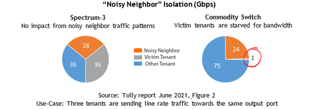
Thenoisy neighbor problem crops up in public and private cloud environments, where multiple tenants use a shared resource, like CPU cycles or network bandwidth, and a “noisy neighbor” tenant shows up and hogs those resources.
The result of the noisy neighbor problem could be that one tenant can degrade the experience of another tenant due to the inadequate capability of the switch to isolate between them. A data center switch must protect tenants from the activities of other tenants, both from nefarious attacks as well as noisy neighbors.
The Tolly Group found that the Spectrum-3 switch fully protected each tenant. The competitor switch failed to protect tenants, allowing the bandwidth of some tenants to be victimized and get fully starved by the traffic pattern of the noisy neighbor.
When scaling out multitenant environments, Spectrum-3 protected each tenant. However, the noisy neighbor problem-scale was way bigger with the commodity switch and can be expanded to half the total number of switch ports. In other words, up to 70 ports can be victimized and starved.
If a switch is not capable of protecting tenants from a noisy neighbor, that switch is not matching a basic requirement from a cloud fabric switch.
Figure 2. Noisy neighbor isolation
(ALT: With Spectrum-3, there is no effect from noisy neighbor traffic patterns. With the commodity switch, victim tenants are starved for bandwidth.)
Storage performance
Today, most storage traffic in the data center runs on Ethernet. More specifically, storage typically uses 9-KB jumbo frames. As a result, this packet size has become more important than ever, and most every switch now supports a default packet size of 9 KB.
However, just because a typical data center switch supports 9-KB packets, doesn’t mean they are optimized for storage workloads. To measure and compare the storage performance levels of each switch, The Tolly Group used 9 KB packets with standard network test tools from IXIA.
The Tolly Group found that Spectrum-3 provided predictable and fair performance across all storage nodes in all cases. The commodity switch showed unfair traffic sharing with 9-KB packets, forcing one storage node to run 17x slower than the other storage nodes. These unpredictable results harshly affect storage performance.
This has real-world implications. Think about the time it takes to run a storage backup. What if your planned and expected 2-hour backup time starts taking 34 hours to complete?
Mixed application performance
Most data centers run many different applications, each with their own packet sizes. Even a single application uses a variety of packet sizes. Adding in control traffic patterns, you will probably end up encountering an even greater variety of packet sizes on your fabric.
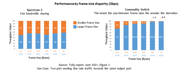
The Tolly Group found that Spectrum-3 provided fairness regardless of the packet size, while the commodity switch tended to starve applications that used smaller packet sizes. Even worse, as the difference in packet sizes increased, the worse it got for the smaller packets.
Figure 3. Performance by frame size disparity
For the commodity switch, mixed packet size starvation adversely affects the cloud, storage, and distributed workloads.
But why?
Architecture. Simple as that.
The Spectrum switches have a modern fully shared buffer architecture and flexible pipeline architecture that were designed to optimize data center application performance and security. For more information about the results, download the new Tolly Group Performance Evaluation report. It explains the architecture of Spectrum switches and commodity switches, along with their advantages and disadvantages.
Architecture is indeed a zero-sum game. However, unlike many other vendors, NVIDIA develops both the ASIC and the switch. As a result, we have managed to eliminate tradeoffs and provide the superior results that The Tolly Group has verified.
The latest update to NVIDIA Nsight Systems is now available and introduces several improvements aimed to enhance the profiling experience.
The latest update to NVIDIA Nsight Systems—a performance analysis tool—is now available for download. Designed to help developers tune and scale software across CPUs and GPUs, this release introduces several improvements aimed to enhance the profiling experience.
Nsight Systems is part of the powerful debugging and profiling NVIDIA Nsight Tools suite. A developer can start with Nsight Systems for overall system view and avoid picking less efficient optimizations based on assumptions and false-positive indicators.
2021.4 Highlights Include:
Windows ISRs and DPCs trace
Windows GPU hardware-based scheduling trace
Windows Direct3D12 and Vulkan correlation to WDDM events
NVTX event categorization support – to enable viewing of categories in isolated rows
Multi-report loading for multinode, VM, container, rank, and process investigations
Nsight system 2021.4 added features to help users understand how timing of other range-based events are affected by the OS interruptions to better account for jitter in statistics or consider binding their processes and threads to core with less frequent ISR and DPC processing.
Figure 1. Windows interrupt trace lets users see when the kernel is operating within your CPU thread.
This release also added data capture that will help users understand when, where, and how deep packets are queued.
Figure 2. Improved graphics correlation allows users to explicitly follow API work submissions through WDDM queue packets and to their GPU workloads, rather than inferring it via timing.
If you are an nvprof or NVIDIA Visual Profiler user, be sure to read the blog posts about migrating to their successors, Nsight Systems, and Nsight Compute.
NVIDIA delivers the best results in AI inference using either x86 or Arm-based CPUs, according to benchmarks released today. It’s the third consecutive time NVIDIA has set records in performance and energy efficiency on inference tests from MLCommons, an industry benchmarking group formed in May 2018. And it’s the first time the data-center category tests Read article >
● Large-scale GPU-based simulation can enable robot learning in simulation, and such solutions can be transferred to real robots without the need for physical access to the robots. This work combines the benefits of IsaacGym-based reinforcement learning for a three-finger in-hand manipulation task and transfers the learned policy to a remote real-world counterpart.
A critical question to ask when designing a machine learning–based solution is, “What’s the resource cost of developing this solution?” There are typically many factors that go into an answer: time, developer skill, and computing resources. It’s rare that a researcher can maximize all these aspects, so optimizing the solution development process is critical. This problem is further aggravated in robotics, as each task typically requires a completely unique solution that involves a nontrivial amount of handcrafting from an expert.
Typical robotics solutions take weeks, if not months, to develop and test. Dexterous, multifinger object manipulation has been one of the long-standing challenges in control and learning for robot manipulation. For more information, see the following papers:
While challenges in high-dimensional control for locomotion as well as image-based object manipulation with simplified grippers have made remarkable progress in the last 5 years, multifinger dexterous manipulation remains a high-impact yet hard-to-crack problem. This challenge is due to a combination of issues:
High-dimensional coordinated control
Inefficient simulation platforms
Uncertainty in observations and control in real-robot operation
Lack of robust and cost-effective hardware platforms
These challenges coupled with lack of availability of large-scale compute and robotic hardware has limited diversity among the teams attempting to address these problems.
Our goal in this effort is to present a path for democratization of robot learning and a viable solution through large-scale simulation and robotics-as-a-service. We focus on six degrees of freedom (6DoF) object manipulation by using a dexterous multifinger manipulator as a case study. We show how large-scale simulation done on a desktop-grade GPU and with cloud-based robotics can enable roboticists to perform research in robotic learning with modest resources.
While several efforts in in-hand manipulation have attempted to build robust systems, one of the most impressive demonstrations came a few years ago from a team at OpenAI that built a system termed Dactyl. It was an impressive feat of engineering to achieve multiobject in-hand reposing with a shadow hand.
However, it was remarkable not only for the final performance but also in the amount of compute and engineering effort to build this demo. As per public estimates, it used 13,000 years of computing and the hardware itself was costly and yet required repeated interventions. The immense resource requirement effectively prevented others from reproducing this result and as a result building on it.
In this post, we show that our systems effort is a path to address this resource inequality. A similar result can now be achieved in under a day using a single desktop-grade GPU and CPU.
Complexity of standard pose representations in the context of reinforcement learning
During the initial experimentation, we followed previous works in providing our policy with observations based on a 3D Cartesian position plus a four-dimensional quaternion representation of pose to specify the current and target position of the cube. We also fixed the reward based on the L2 norm (position) and angular difference (orientation) between the desired and current pose of the cube. For more information, see the Learning Dexterity OpenAI post and GPU-Accelerated Robotic Simulation for Distributed Reinforcement Learning.
We found this approach to produce unstable reward curves, which were good at optimizing the position portion of the reward, even after adjusting relative weightings.
Figure 1. Training curves on the trifinger manipulation task using a reward function similar to previous works. The nature of the reward makes it difficult for the policy to optimize, particularly achieving an orientation goal.
Inspired by this, we searched for a representation of pose in SO(3) for our 6DoF reposing problem. This would also naturally trade off position and rotation rewards in a way suited to optimization through reinforcement learning.
Closing the Sim2Real gap with remote robots
The problem of access to physical robotic resources was exacerbated by the COVID-19 pandemic. Those previously fortunate enough to have access to robots in their research groups found that the number of people with physical access to the robots was greatly decreased. Those that relied on other institutions to provide the hardware were often alienated completely due to physical distancing restrictions.
Our work demonstrated the feasibility of a robotics-as-a-service (RaaS) approach in tandem with robot learning. A small team of people trained to maintain the robot and a separate team of researchers could upload a trained policy and remotely collect data for postprocessing.
While our team of researchers was primarily based in North America, the physical robot was in Europe. For the duration of the project, our development team was never physically in the same room as the robots on which we were working. Remote access meant that we could not vary the task at hand to make it easier. It also limited the kinds of iteration and experiments that we could do. For example, reasoned system identification was not possible, as our policy ran on a randomly chosen robot in the entire farm.
Despite the lack of physical access, we found that we were able to produce a robust and working policy to solve the 6DoF reposing task through a combination of several techniques:
Realistic GPU-accelerated simulation
Model-free RL
Domain randomization
Task-appropriate representation of pose
Method overview
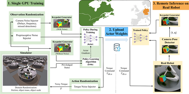
Our system trains using the IsaacGym simulator on 16,384 environments in parallel on a single NVIDIA V100 or NVIDIA RTX 3090 GPU. Inference is then conducted remotely on a TriFinger robot located across the Atlantic in Germany using the uploaded actor weights. The infrastructure on which we perform Sim2Real transfer is provided courtesy of the organizers of the Real Robot Challenge.
Figure 2. Training system flowchart
Collect and process training examples
Using the IsaacGym simulator, we gathered high-throughput experience (~100K samples/sec on an NVIDIA RTX 3090). The sample’s object pose and goal pose are to eight keypoints of the object’s shape. Domain randomizations were applied to the observations and environment parameters to simulate variations in the proprioceptive sensors of the real robots and cameras. These observations, along with some privileged state information from the simulator, were then used to train our policy.
Train the policy
Our policy was trained to maximize a custom reward using the proximal policy optimization (PPO) algorithm. Our reward incentivized the policy to balance the distance of the robot’s fingers from the object, speed of movement, and distance from the object to a specified goal position. It solved the task efficiently, despite being a general formulation applicable broadly across in-hand manipulation applications. The policy output the torques for each of the robot’s motors, which were then passed back into the simulation environment.
Transfer the policy to a real robot and run inference
After we trained the policy, we uploaded it to the controller for the real robot. The cube was tracked on the system using three cameras. We combined proprioceptive information available from the system along with the converted keypoints representation to provide input to the policy. We repeated the camera-based cube-pose observations for subsequent rounds of policy evaluation to enable the policy to take advantage of the higher-frequency proprioceptive data available to the robot. The data collected from the system was then used to determine the success rate of the policy.
The tracking system on the robot currently only supports cubes. However, this could be extended in future to arbitrary objects.
Results
The keypoints representation of pose greatly improves success rate and convergence.
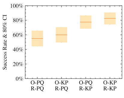
Figure 3. Success rate on the real robot plotted for different trained agents. O-PQ and O-KP stand for position+quaternion and keypoints observations respectively, and R-PQ and R-KP stand for linear+angular and keypoints-based displacements respectively. Each meanmade of N=40 trials and error bars calculated based on an 80% confidence interval.
We demonstrated that the policies that used our keypoint representation, in either the observation provided to the policy or in reward calculation, achieved a higher success rate than using a position+quaternion representation. The highest performance came from the policies that used the alternate representation for both elements.
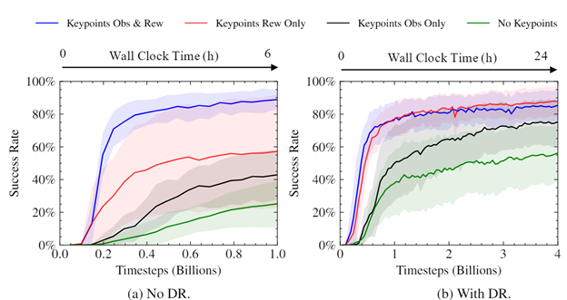
Figure 4. Success rate over the course of training without and with domain randomization. Each curve is the average of five seeds; the shaded areas show standard deviation. Training without DR is shown to 1B steps to verify performance; use of DR didn’t have a large impact on simulation success rates after initial training.
We performed experiments to see how the use of keypoints impacted the speed and convergence level of our trained policies. As can be seen, using keypoints as part of the reward considerably sped up training, improved the eventual success rate, and reduced variance between trained policies. The magnitude of the difference was surprising, given the simplicity and generality of using keypoints as part of the reward.
The trained policies can be deployed straight from the simulator to remote real robots (Figure 5).
Figure 5. Real-time video of robot picking up the cube and reposing it in 6DoF
Figure 6 displays an emergent behavior that we’ve termed “dropping and regrasping.” In this maneuver, the robot learns to drop the cube when it is close to the correct position, regrasp it, and pick it back up. This enables the robot to get a stable grasp on the cube in the right position, which leads to more successful attempts. It’s worth noting that this video is in real time and not sped up in any way.
The robot also learns to use the motion of the cube to the correct location in the arena as an opportunity to rotate it on the ground simultaneously. This helps achieve the correct grasp in challenging target locations far from the center of the fingers’ workspace.
Figure 6. A poor grasp leads to the cube slipping. Without being explicitly trained to, the robot has learned how to recover from such falls.
Our policy is also robust towards dropping. The robot can recover from a cube falling out of the hand and retrieve it from the ground.
Robustness to physics and object variations
We found that our policy was robust to variations in environment parameters in simulation. For example, it gracefully handled scaling up and down of the cube by ranges far exceeding randomization.
Figure 7. (Left) A cube scaled down by a factor of 2 (left) being successfully manipulated by the robot
Figure 7. (Right) A cube scaled up by a factor of 2 being successfully manipulated by the robot
Surprisingly, we found that our policies were able to generalize 0-shot to other objects, for example, a cuboid or a ball.
Figure 8. (Left) A cuboid being successfully manipulated by the robot.
Figure 8. (Right) A sphere being successfully manipulated by the robot.
Generalization in scale and object is taking place due to the policy’s own robustness. We do not give it any shape information. The keypoints remain in the same place as they would on a cube.
Figure 9. Example of a successful completion of the manipulation task with the keypoints visualized
Conclusion
Our method shows a viable path for robot learning through large-scale, GPU-based simulation. In this post, we showed you how it is possible to train a policy using moderate levels of computational resources (desktop-level compute) and transfer it to a remote robot. We also showed that these policies are robust to a variety of changes in the environment and the object being manipulated. We hope our work can serve as a platform for researchers going forward.
NVIDIA has also announced broad support for the Robotics Operating System (ROS) with Open Robotics. This important Isaac ROS announcement underlines how NVIDIA AI perception technologies accelerate AI utilization in the ROS community to help roboticists, researchers, and robot users looking to develop, test, and manage next-generation, AI-based robots.
This work was led by University of Toronto in collaboration with NVIDIA, Vector Institute, MPI, ETH, and Snap. We would like to thank Vector Institute for computing support, as well as the CIFAR AI Chair for research support to Animesh Garg.
A look at NVIDIA inference performance as measured by the MLPerf Inference 1.1 benchmark. NVIDIA delivers leadership performance across all workloads and scenarios, and in an industry-first, has delivered results on an Arm-based server in the data center category. MLPerf Inference 1.1 tests performance and power efficiency across usages including computer vision, natural language processing and recommender systems.
AI continues to drive breakthrough innovation across industries, including consumer Internet, healthcare and life sciences, financial services, retail, manufacturing, and supercomputing. Researchers continue to push the boundaries of what’s possible with rapidly evolving models that are growing in size, complexity, and diversity. In addition, many of these complex, large-scale models need to deliver results in real time for AI-powered services like chatbots, digital assistants, and fraud detection to name a few.
Given the wide array of uses for AI inference, evaluating performance poses numerous challenges for developers and infrastructure managers. For AI inference on data center, edge, and mobile platforms, MLPerf Inference 1.1 is an industry-standard benchmark that measures performance across computer vision, medical imaging, natural language, and recommender systems. These benchmarks were developed by a consortium of AI industry leaders, providing the most comprehensive set of peer-reviewed performance data available today, both for AI training and inference.
To perform well on the wide array of tests in this benchmark requires a full-stack platform with great ecosystem support, both for frameworks and networks. NVIDIA was the only company to make submissions for all data center and edge tests and deliver leading performance across the board.
One of the great byproducts of this work is that many of these optimizations have found their way into inference developer tools like TensorRT and NVIDIA Triton. The TensorRT SDK for high-performance deep learning inference includes a deep learning inference optimizer and runtime that delivers low latency and high throughput for deep learning inference applications.
The Triton Inference Server software simplifies the deployment of AI models at scale in production. This open-source inference serving software enables teams to deploy trained AI models from any framework from local storage or cloud platform on any GPU– or CPU-based infrastructure.
By the numbers
Across the board in both data center and edge categories, NVIDIA took top spots in performance tests with the NVIDIA A100 Tensor Core GPU and all but one with our NVIDIA A30 Tensor Core GPU. Over the last year since results for MLPerf Inference 0.7 were published, NVIDIA delivered up to 50% more performance from software improvements alone.
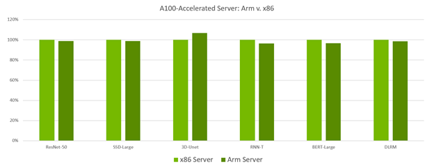
In another industry first, NVIDIA made the first-ever datacenter category submissions with a GPU-accelerated Arm-based server, which supported all workloads and delivered results equal to those seen on a similarly configured x86-based server. These new Arm-based submissions set new performance world records for GPU-accelerated Arm servers. This marks an important milestone for these platforms as they have now proven themselves in a peer-reviewed industry-standard benchmark to deliver market-leading performance. It also shows the performance, versatility, and readiness of the NVIDIA Arm software ecosystem for tackling computing challenges in the data center.
Figure 1. Arm-based server using Ampere Altra CPUs delivers performance on par with similarly equipped x86-based server
MLPerf v1.1 Inference Closed; Per-accelerator performance derived from the best MLPerf results for respective submissions using reported accelerator count in Data Center Offline. x86 Server: 1.1-034, Arm Server: 1.1-033 MLPerf name and logo are trademarks. Source: www.mlcommons.org.
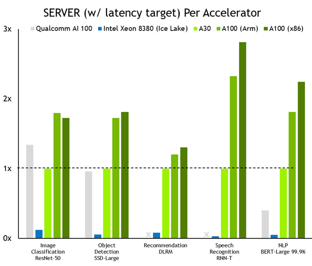
A look at overall performance shows that NVIDIA leads across the board. Figure 2 shows results for the server scenario, where inference work for the system-under-test is generated using a Poisson distribution to model real-world workload patterns more closely.
Figure 2. NVIDIA performance compared to CPU-only servers
MLPerf v1.1 Inference Closed; Per-accelerator performance derived from the best MLPerf results for respective submissions using reported accelerator count in Data Center Offline and Server. Qualcomm AI 100: 1.1-057 and 1.1-058, Intel Xeon 8380: 1.1-023 and 1.1-024, NVIDIA A30: 1.1-43, NVIDIA A100 (Arm): 1.1-033, NVIDIA A100 (x86): 1.1-047. MLPerf name and logo are trademarks. Source: www.mlcommons.org.
NVIDIA outperforms CPU-only servers across the board, by as much as 104x. This performance advantage translates into an ability to run inference on larger, more complex models, as well as multiple models run in real-time jobs in conversational AI, recommender systems, and digital assistants.
Optimizations behind the results
Our engineering team implemented several optimizations to make these great results possible. For starters, all these results—both for Arm–based and x86-based servers—were generated using TensorRT 8, which is now generally available. Of particular interest was the use of non-power-of-two kernels, which was implemented to speed up workloads such as the BERT-Large Single Stream scenario test.
NVIDIA submissions take advantage of the new host policy feature added to the NVIDIA Triton Inference server. You can specify a host policy while configuring the NVIDIA Triton server that enables thread and memory pinning in the server application. With this feature, NVIDIA Triton can specify the optimal location of inputs for every GPU in the system. The optimal location can be based on the non-uniform memory architecture (NUMA) configuration of the system, in which case there is a query sample library on every NUMA node.
You can also use the host policy to enable the start_from_device configuration setting, where the server will pick up the input on the GPU chosen for execution. This setting can also land network inputs directly into GPU memory, entirely bypassing the CPU and system memory copies.
Inference power trio: TensorRT, NVIDIA Triton, and NGC
NVIDIA inference leadership comes from building the most performant AI accelerators, both for training and inference. But just as important is the NVIDIA end-to-end, full-stack software ecosystem that supports all AI frameworks and more than 800 HPC applications.
All this software is available at NGC, the NVIDIA hub with GPU-optimized software for deep learning, machine learning, and HPC. NGC takes care of all the plumbing so data scientists, developers, and researchers can focus on building solutions, gathering insights, and delivering business value.
NGC is freely available through the marketplace of your preferred cloud provider. There, you can find the latest versions of both TensorRT as well as NVIDIA Triton, both of which were instrumental in producing the latest MLPerf Inference 1.1 results.
For more information about the NVIDIA inference platform, see the Inference Technical Overview paper that covers the trends in AI inference, challenges around deploying AI applications, and details of inference development tools and application frameworks.
Posted by Jing Yu Koh, Research Engineer and Peter Anderson, Senior Research Scientist, Google Research
When a person navigates around an unfamiliar building, they take advantage of many visual, spatial and semantic cues to help them efficiently reach their goal. For example, even in an unfamiliar house, if they see a dining area, they can make intelligent predictions about the likely location of the kitchen and lounge areas, and therefore the expected location of common household objects. For robotic agents, taking advantage of semantic cues and statistical regularities in novel buildings is challenging. A typical approach is to implicitly learn what these cues are, and how to use them for navigation tasks, in an end-to-end manner via model-free reinforcement learning. However, navigation cues learned in this way are expensive to learn, hard to inspect, and difficult to re-use in another agent without learning again from scratch.
People navigating in unfamiliar buildings can take advantage of visual, spatial and semantic cues to predict what’s around a corner. A computational model with this capability is a visual world model.
An appealing alternative for robotic navigation and planning agents is to use a world model to encapsulate rich and meaningful information about their surroundings, which enables an agent to make specific predictions about actionable outcomes within their environment. Such models have seen widespread interest in robotics, simulation, and reinforcement learning with impressive results, including finding the first known solution for a simulated 2D car racing task, and achieving human-level performance in Atari games. However, game environments are still relatively simple compared to the complexity and diversity of real-world environments.
In “Pathdreamer: A World Model for Indoor Navigation”, published at ICCV 2021, we present a world model that generates high-resolution 360º visual observations of areas of a building unseen by an agent, using only limited seed observations and a proposed navigation trajectory. As illustrated in the video below, the Pathdreamer model can synthesize an immersive scene from a single viewpoint, predicting what an agent might see if it moved to a new viewpoint or even a completely unseen area, such as around a corner. Beyond potential applications in video editing and bringing photos to life, solving this task promises to codify knowledge about human environments to benefit robotic agents navigating in the real world. For example, a robot tasked with finding a particular room or object in an unfamiliar building could perform simulations using the world model to identify likely locations before physically searching anywhere. World models such as Pathdreamer can also be used to increase the amount of training data for agents, by training agents in the model.
Provided with just a single observation (RGB, depth, and segmentation) and a proposed navigation trajectory as input, Pathdreamer synthesizes high resolution 360º observations up to 6-7 meters away from the original location, including around corners. For more results, please refer to the full video.
How Does Pathdreamer Work? Pathdreamer takes as input a sequence of one or more previous observations, and generates predictions for a trajectory of future locations, which may be provided up front or iteratively by the agent interacting with the returned observations. Both inputs and predictions consist of RGB, semantic segmentation, and depth images. Internally, Pathdreamer uses a 3D point cloud to represent surfaces in the environment. Points in the cloud are labelled with both their RGB color value and their semantic segmentation class, such as wall, chair or table.
To predict visual observations in a new location, the point cloud is first re-projected into 2D at the new location to provide ‘guidance’ images, from which Pathdreamer generates realistic high-resolution RGB, semantic segmentation and depth. As the model ‘moves’, new observations (either real or predicted) are accumulated in the point cloud. One advantage of using a point cloud for memory is temporal consistency — revisited regions are rendered in a consistent manner to previous observations.
Internally, Pathdreamer represents surfaces in the environment via a 3D point cloud containing both semantic labels (top) and RGB color values (bottom). To generate a new observation, Pathdreamer ‘moves’ through the point cloud to the new location and uses the re-projected point cloud image for guidance.
To convert guidance images into plausible, realistic outputs Pathdreamer operates in two stages: the first stage, the structure generator, creates segmentation and depth images, and the second stage, the image generator, renders these into RGB outputs. Conceptually, the first stage provides a plausible high-level semantic representation of the scene, and the second stage renders this into a realistic color image. Both stages are based on convolutional neural networks.
Pathdreamer operates in two stages: the first stage, the structure generator, creates segmentation and depth images, and the second stage, the image generator, renders these into RGB outputs. The structure generator is conditioned on a noise variable to enable the model to synthesize diverse scenes in areas of high uncertainty.
Diverse Generation Results In regions of high uncertainty, such as an area predicted to be around a corner or in an unseen room, many different scenes are possible. Incorporating ideas from stochastic video generation, the structure generator in Pathdreamer is conditioned on a noise variable, which represents the stochastic information about the next location that is not captured in the guidance images. By sampling multiple noise variables, Pathdreamer can synthesize diverse scenes, allowing an agent to sample multiple plausible outcomes for a given trajectory. These diverse outputs are reflected not only in the first stage outputs (semantic segmentation and depth images), but in the generated RGB images as well.
Pathdreamer is capable of generating multiple diverse and plausible images for regions of high uncertainty. Guidance images on the leftmost column represent pixels that were previously seen by the agent. Black pixels represent regions that were previously unseen, for which Pathdreamer renders diverse outputs by sampling multiple random noise vectors. In practice, the generated output can be informed by new observations as the agent navigates the environment.
<!–
Pathdreamer is capable of generating multiple diverse and plausible images for regions of high uncertainty. Guidance images on the leftmost column represent pixels that were previously seen by the agent. Black pixels represent regions that were previously unseen, for which Pathdreamer renders diverse outputs by sampling multiple random noise vectors. In practice, the generated output can be informed by new observations as the agent navigates the environment.
–>
Pathdreamer is trained with images and 3D environment reconstructions from Matterport3D, and is capable of synthesizing realistic images as well as continuous video sequences. Because the output imagery is high-resolution and 360º, it can be readily converted for use by existing navigation agents for any camera field of view. For more details and to try out Pathdreamer yourself, we recommend taking a look at our open source code.
Application to Visual Navigation Tasks As a visual world model, Pathdreamer shows strong potential to improve performance on downstream tasks. To demonstrate this, we apply Pathdreamer to the task of Vision-and-Language Navigation (VLN), in which an embodied agent must follow a natural language instruction to navigate to a location in a realistic 3D environment. Using the Room-to-Room (R2R) dataset, we conduct an experiment in which an instruction-following agent plans ahead by simulating many possible navigable trajectory through the environment, ranking each against the navigation instructions, and choosing the best ranked trajectory to execute. Three settings are considered. In the Ground-Truth setting, the agent plans by interacting with the actual environment, i.e. by moving. In the Baseline setting, the agent plans ahead without moving by interacting with a navigation graph that encodes the navigable routes within the building, but does not provide any visual observations. In the Pathdreamer setting, the agent plans ahead without moving by interacting with the navigation graph and also receives corresponding visual observations generated by Pathdreamer.
When planning ahead for three steps (approximately 6m), in the Pathdreamer setting the VLN agent achieves a navigation success rate of 50.4%, significantly higher than the 40.6% success rate in the Baseline setting without Pathdreamer. This suggests that Pathdreamer encodes useful and accessible visual, spatial and semantic knowledge about real-world indoor environments. As an upper bound illustrating the performance of a perfect world model, under the Ground-Truth setting (planning by moving) the agent’s success rate is 59%, although we note that this setting requires the agent to expend significant time and resources to physically explore many trajectories, which would likely be prohibitively costly in a real-world setting.
We evaluate several planning settings for an instruction-following agent using the Room-to-Room (R2R) dataset. Planning ahead using a navigation graph with corresponding visual observations synthesized by Pathdreamer (Pathdreamer setting) is more effective than planning ahead using the navigation graph alone (Baseline setting), capturing around half the benefit of planning ahead using a world model that perfectly matches reality (Ground-Truth setting).
Conclusions and Future Work These results showcase the promise of using world models such as Pathdreamer for complicated embodied navigation tasks. We hope that Pathdreamer will help unlock model-based approaches to challenging embodied navigation tasks such as navigating to specified objects and VLN.
Applying Pathdreamer to other embodied navigation tasks such as Object-Nav, continuous VLN, and street-level navigation are natural directions for future work. We also envision further research on improved architecture and modeling directions for the Pathdreamer model, as well as testing it on more diverse datasets, including but not limited to outdoor environments. To explore Pathdreamer in more detail, please visit our GitHub repository.
Acknowledgements This project is a collaboration with Jason Baldridge, Honglak Lee, and Yinfei Yang. We thank Austin Waters, Noah Snavely, Suhani Vora, Harsh Agrawal, David Ha, and others who provided feedback throughout the project. We are also grateful for general support from Google Research teams. Finally, we thank Tom Small for creating the animation in the third figure.

 Independent IT lab The Tolly Group compared the cloud, AI, and storage performance of an NVIDIA Ethernet switch to the performance of a comparable switch built with commodity silicon.
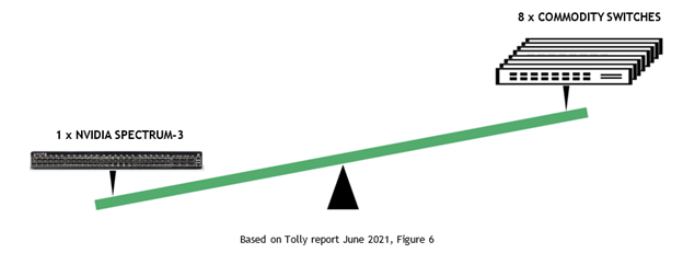
 The latest update to NVIDIA Nsight Systems is now available and introduces several improvements aimed to enhance the profiling experience.
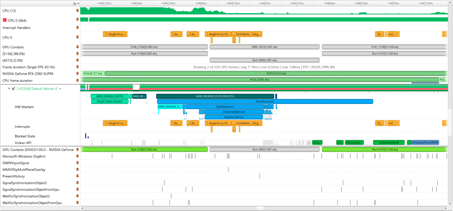

 ● Large-scale GPU-based simulation can enable robot learning in simulation, and such solutions can be transferred to real robots without the need for physical access to the robots. This work combines the benefits of IsaacGym-based reinforcement learning for a three-finger in-hand manipulation task and transfers the learned policy to a remote real-world counterpart.
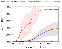
 A look at NVIDIA inference performance as measured by the MLPerf Inference 1.1 benchmark. NVIDIA delivers leadership performance across all workloads and scenarios, and in an industry-first, has delivered results on an Arm-based server in the data center category. MLPerf Inference 1.1 tests performance and power efficiency across usages including computer vision, natural language processing and recommender systems.