New research creates a low-cost and easy-to-use machine learning model to analyze streams of data from earth-imaging satellites.
New research from a group of scientists at UC Berkeley is giving data-poor regions across the globe the power to analyze data-rich satellite imagery. The study, published in Nature Communications, develops a machine learning model resource-constrained organizations and researchers can use to draw out regional socioeconomic and environmental information. Being able to evaluate local resources remotely could help guide effective interventions and benefit communities globally.
“We saw that many researchers—ourselves included—were passing up on this valuable data source because of the complexities and upfront costs associated with building computer vision pipelines to translate raw pixel values into useful information. We thought that there might be a way to make this information more accessible while maintaining the predictive skill offered by state-of-the-art approaches. So, we set about constructing a way to do this,” said coauthor Ian Bolliger, who worked on the study while pursuing a PhD in Energy and Resources at UC Berkeley.
At any given time, hundreds of image-collecting satellites circle the earth, sending massive amounts of information to databases daily. This data holds valuable insight into global challenges, including health, economic, and environmental conditions—even offering a look into data-poor and remote regions.
Combining satellite imagery with machine learning (SIML) has become an effective tool for turning these raw data streams into usable information. Researchers have used SIML on a broad-range of studies, from calculating poverty rates, to water availability, to educational access. However, most SIML projects capture information on a narrow topic, creating data tailored to a specific study and location.
The researchers sought to create an accessible system capable of analyzing and organizing satellite images from multiple sources while lowering compute requirements. The tool they created, called the Multi-Task Observation using Satellite Imagery & Kitchen Sinks (MOSAIKS), does this by using a relatively simpler and more efficient unsupervised machine learning algorithm.
“We designed MOSAIKS keeping in mind that a single satellite image simultaneously holds information about many different prediction variables (like forest cover or population density.) We chose to use an unsupervised embedding of the imagery to create a statistical summary of each image. The unsupervised nature of the featurization step makes the learning and prediction steps of the pipeline very fast, while the specifics of how those features are computed from imagery are well suited to satellite image data,” said coauthor Esther Rolf, a Ph.D. student in computer science at Berkeley.
To develop the model, the researchers used CUDA-accelerated NVIDIA V100 Tensor Core GPUs on AWS. The publicly available CodeOcean capsule, which provides code, compute, and storage, for anyone to interactively run, uses NVIDIA GPUs.
Figure 1. Training data (left) and predictions using a single featurization of daytime imagery (right). Insets (far right) marked by black squares in global maps. Training sample is a uniform random sampling of 1,000,000 land grid cells, 498,063 for which imagery were available and could be matched to task labels.
“We want policymakers in resource-constrained settings and without specialized computational expertise to be able to painlessly gather satellite imagery, build a model of a variable they care about (say, the presence of adequate sanitation systems), and test whether this model is actually performing well. If they can do this, it will dramatically improve the usefulness of this information in implementing policy objectives,” Bolliger said.
Currently the team is developing and testing a public-facing web interface tool, making it easy for people to query for MOSAIKS features in user-specified locations. The researchers encourage interested researchers to sign up for the beta version.
Posted by Kihyuk Sohn and Chun-Liang Li, Research Scientists, Google Cloud
Anomaly detection (sometimes called outlier detection or out-of-distribution detection) is one of the most common machine learning applications across many domains, from defect detection in manufacturing to fraudulent transaction detection in finance. It is most often used when it is easy to collect a large amount of known-normal examples but where anomalous data is rare and difficult to find. As such, one-class classification, such as one-class support vector machine (OC-SVM) or support vector data description (SVDD), is particularly relevant to anomaly detection because it assumes the training data are all normal examples, and aims to identify whether an example belongs to the same distribution as the training data. Unfortunately, these classical algorithms do not benefit from the representation learning that makes machine learning so powerful. On the other hand, substantial progress has been made in learning visual representations from unlabeled data via self-supervised learning, including rotation prediction and contrastive learning. As such, combining one-class classifiers with these recent successes in deep representation learning is an under-explored opportunity for the detection of anomalous data.
A Two-Stage Framework for Deep One-Class Classification While end-to-end learning has demonstrated success in many machine learning problems, including deep learning algorithm designs, such an approach for deep one-class classifiers often suffer from degeneration in which the model outputs the same results regardless of the input.
To combat this, we apply a two stage framework. In the first stage, the model learns deep representations with self-supervision. In the second stage, we adopt one-class classification algorithms, such as OC-SVM or kernel density estimator, using the learned representations from the first stage. This 2-stage algorithm is not only robust to degeneration, but also enables one to build more accurate one-class classifiers. Furthermore, the framework is not limited to specific representation learning and one-class classification algorithms — that is, one can easily plug-and-play different algorithms, which is useful if any advanced approaches are developed.
A deep neural network is trained to generate the representations of input images via self-supervision. We then train one-class classifiers on the learned representations.
Semantic Anomaly Detection We test the efficacy of our 2-stage framework for anomaly detection by experimenting with two representative self-supervised representation learning algorithms, rotation prediction and contrastive learning.
Rotation prediction refers to a model’s ability to predict the rotated angles of an input image. Due to its promising performance in other computer vision applications, the end-to-end trained rotation prediction network has been widelyadopted for one-class classification research. The existing approach typically reuses the built-in rotation prediction classifier for learning representations to conduct anomaly detection, which is suboptimal because those built-in classifiers are not trained for one-class classification.
In contrastive learning, a model learns to pull together representations from transformed versions of the same image, while pushing representations of different images away. During training, as images are drawn from the dataset, each is transformed twice with simple augmentations (e.g., random cropping or color changing). We minimize the distance of the representations from the same image to encourage consistency and maximize the distance between different images. However, usual contrastive learning converges to a solution where all the representations of normal examples are uniformly spread out on a sphere. This is problematic because most of the one-class algorithms determine the outliers by checking the proximity of a tested example to the normal training examples, but when all the normal examples are uniformly distributed in an entire space, outliers will always appear close to some normal examples.
To resolve this, we propose distribution augmentation (DA) for one-class contrastive learning. The idea is that instead of learning representations from the training data only, the model learns from the union of the training data plus augmented training examples, where the augmented examples are considered to be different from the original training data. We employ geometric transformations, such as rotation or horizontal flip, for distribution augmentation. With DA, the training data is no longer uniformly distributed in the representation space because some areas are occupied by the augmented data.
Left: Illustrated examples of perfect uniformity from the standard contrastive learning. Right: The reduced uniformity by the proposed distribution augmentation (DA), where the augmented data occupy the space to avoid the uniform distribution of the inlier examples (blue) throughout the whole sphere.
We evaluate the performance of one-class classification in terms of the area under receiver operating characteristic curve (AUC) on the commonly used datasets in computer vision, including CIFAR10 and CIFAR-100, Fashion MNIST, and Cat vs Dog. Images from one class are given as inliers and those from remaining classes are given as outliers. For example, we see how well cat images are detected as anomalies when dog images are inliers.
CIFAR-10
CIFAR-100
f-MNIST
Cat v.s. Dog
Ruff et al. (2018)
64.8
–
–
–
Golan and El-Yaniv (2018)
86.0
78.7
93.5
88.8
Bergman and Hoshen (2020)
88.2
–
94.1
–
Hendrycks et al. (2019)
90.1
–
–
–
Huang et al. (2019)
86.6
78.8
93.9
–
2-stage framework: rotation prediction
91.3±0.3
84.1±0.6
95.8±0.3
86.4±0.6
2-stage framework: contrastive (DA)
92.5±0.6
86.5±0.7
94.8±0.3
89.6±0.5
Performance comparison of one-class classification methods. Values are the mean AUCs and their standard deviation over 5 runs. AUC ranges from 0 to 100, where 100 is perfect detection.
Given the suboptimal built-in rotation prediction classifiers typically used for rotation prediction approaches, it’s notable that simply replacing the built-in rotation classifier used in the first stage for learning representations with a one-class classifier at the second stage of the proposed framework significantly boosts the performance, from 86 to 91.3 AUC. More generally, the 2-stage framework achieves state-of-the-art performance on all of the above benchmarks.
With classic OC-SVM, which learns the area boundary of representations of normal examples, the 2-stage framework results in higher performance than existing works as measured by image-level AUC.
Texture Anomaly Detection for Industrial Defect Detection In many real-world applications of anomaly detection, the anomaly is often defined by localized defects instead of entirely different semantics (i.e., being different in general). For example, the detection of texture anomalies is useful for detecting various kinds of industrial defects.
The examples of semantic anomaly detection and defect detection. In semantic anomaly detection, the inlier and outlier are different in general, (e.g., one is a dog, the other a cat). In defect detection, the semantics for inlier and outlier are the same (e.g., they are both tiles), but the outlier has a local anomaly.
While learning representations with rotation prediction and distribution-augmented contrastive learning have demonstrated state-of-the-art performance on semantic anomaly detection, those algorithms do not perform well on texture anomaly detection. Instead, we explored different representation learning algorithms that better fit the application.
In our second paper, we propose a new self-supervised learning algorithm for texture anomaly detection. The overall anomaly detection follows the 2-stage framework, but the first stage, in which the model learns deep image representations, is specifically trained to predict whether the image is augmented via a simple CutPaste data augmentation. The idea of CutPaste augmentation is simple — a given image is augmented by randomly cutting a local patch and pasting it back to a different location of the same image. Learning to distinguish normal examples from CutPaste-augmented examples encourages representations to be sensitive to local irregularity of an image.
The illustration of learning representations by predicting CutPaste augmentations. Given an example, the CutPaste augmentation crops a local patch, then pasties it to a randomly selected area of the same image. We then train a binary classifier to distinguish the original image and the CutPaste augmented image.
We use MVTec, a real-world defect detection dataset with 15 object categories, to evaluate the approach above.
Image-level anomaly detection performance (in AUC) on the MVTec benchmark.
Besides image-level anomaly detection, we use the CutPaste method to locate where the anomaly is, i.e., “patch-level” anomaly detection. We aggregate the patch anomaly scores via upsampling with Gaussian smoothing and visualize them in heatmaps that show where the anomaly is. Interestingly, this provides decently improved localization of anomalies. The below table shows the pixel-level AUC for localization evaluation.
Pixel-level anomaly localization performance (in AUC) comparison between different algorithms on the MVTec benchmark.
Conclusion In this work we introduce a novel 2-stage deep one-class classification framework and emphasize the importance of decoupling building classifiers from learning representations so that the classifier can be consistent with the target task, one-class classification. Moreover, this approach permits applications of various self-supervised representation learning methods, attaining state-of-the-art performance on various applications of visual one-class classification from semantic anomaly to texture defect detection. We are extending our efforts to build more realistic anomaly detection methods under the scenario where training data is truly unlabeled.
Acknowledgements We gratefully acknowledge the contribution from other co-authors, including Jinsung Yoon, Minho Jin and Tomas Pfister. We release the code in our GitHub repository.
I have a problem using LSTM from keras. When I try to train the model, the training stops at “Epoch 1/50” and never progresses. The program just stops with a Process finished code and shows no error messages regarding the missing training.
The problem only occurs when I try to use LSTM’s default parameters. So if I for example give a new activation argument with such as “relu” then it works fine?
It seems to be on my local computer the problem pertains as the code can run on Colab with and without default parameters, but for some reason I can not be allowed to train the model at all. This is especially frustrating as there are no error messages displayed.
I really hope there is a skilled person who can help or guide me in the right direction with this problem.
Thanks 🙂
import tensorflow as tf
from tensorflow.keras.models import Sequential
from tensorflow.keras.layers import Dense, Dropout, LSTM, InputLayer
2021-08-27 10:20:22.799484: I tensorflow/stream_executor/platform/default/dso_loader.cc:53] Successfully opened dynamic library cudart64_110.dll 2021-08-27 10:20:26.443509: I tensorflow/stream_executor/platform/default/dso_loader.cc:53] Successfully opened dynamic library nvcuda.dll 2021-08-27 10:20:26.488972: I tensorflow/core/common_runtime/gpu/gpu_device.cc:1733] Found device 0 with properties: pciBusID: 0000:01:00.0 name: NVIDIA GeForce RTX 2060 computeCapability: 7.5 coreClock: 1.2GHz coreCount: 30 deviceMemorySize: 6.00GiB deviceMemoryBandwidth: 245.91GiB/s 2021-08-27 10:20:26.489580: I tensorflow/stream_executor/platform/default/dso_loader.cc:53] Successfully opened dynamic library cudart64_110.dll 2021-08-27 10:20:26.532650: I tensorflow/stream_executor/platform/default/dso_loader.cc:53] Successfully opened dynamic library cublas64_11.dll 2021-08-27 10:20:26.533109: I tensorflow/stream_executor/platform/default/dso_loader.cc:53] Successfully opened dynamic library cublasLt64_11.dll 2021-08-27 10:20:26.559639: I tensorflow/stream_executor/platform/default/dso_loader.cc:53] Successfully opened dynamic library cufft64_10.dll 2021-08-27 10:20:26.565224: I tensorflow/stream_executor/platform/default/dso_loader.cc:53] Successfully opened dynamic library curand64_10.dll 2021-08-27 10:20:26.637251: I tensorflow/stream_executor/platform/default/dso_loader.cc:53] Successfully opened dynamic library cusolver64_11.dll 2021-08-27 10:20:26.660612: I tensorflow/stream_executor/platform/default/dso_loader.cc:53] Successfully opened dynamic library cusparse64_11.dll 2021-08-27 10:20:26.661815: I tensorflow/stream_executor/platform/default/dso_loader.cc:53] Successfully opened dynamic library cudnn64_8.dll 2021-08-27 10:20:26.662201: I tensorflow/core/common_runtime/gpu/gpu_device.cc:1871] Adding visible gpu devices: 0 2021-08-27 10:20:26.662770: I tensorflow/core/platform/cpu_feature_guard.cc:142] This TensorFlow binary is optimized with oneAPI Deep Neural Network Library (oneDNN) to use the following CPU instructions in performance-critical operations: AVX AVX2 To enable them in other operations, rebuild TensorFlow with the appropriate compiler flags. 2021-08-27 10:20:26.664656: I tensorflow/core/common_runtime/gpu/gpu_device.cc:1733] Found device 0 with properties: pciBusID: 0000:01:00.0 name: NVIDIA GeForce RTX 2060 computeCapability: 7.5 coreClock: 1.2GHz coreCount: 30 deviceMemorySize: 6.00GiB deviceMemoryBandwidth: 245.91GiB/s 2021-08-27 10:20:26.665660: I tensorflow/core/common_runtime/gpu/gpu_device.cc:1871] Adding visible gpu devices: 0 2021-08-27 10:20:27.284225: I tensorflow/core/common_runtime/gpu/gpu_device.cc:1258] Device interconnect StreamExecutor with strength 1 edge matrix: 2021-08-27 10:20:27.284551: I tensorflow/core/common_runtime/gpu/gpu_device.cc:1264] 0 2021-08-27 10:20:27.284738: I tensorflow/core/common_runtime/gpu/gpu_device.cc:1277] 0: N 2021-08-27 10:20:27.285152: I tensorflow/core/common_runtime/gpu/gpu_device.cc:1418] Created TensorFlow device (/job:localhost/replica:0/task:0/device:GPU:0 with 3961 MB memory) -> physical GPU (device: 0, name: NVIDIA GeForce RTX 2060, pci bus id: 0000:01:00.0, compute capability: 7.5) 2021-08-27 10:20:28.198186: I tensorflow/compiler/mlir/mlir_graph_optimization_pass.cc:176] None of the MLIR Optimization Passes are enabled (registered 2) Epoch 1/50 2021-08-27 10:20:29.513381: I tensorflow/stream_executor/platform/default/dso_loader.cc:53] Successfully opened dynamic library cudnn64_8.dll Process finished with exit code -1073740791 (0xC0000409)
Healthcare giant Johnson & Johnson is injecting data science across its business to improve its manufacturing, clinical trial enrollment, forecasting and more. “I actually like to call it decision science,” said Jim Swanson, the company’s executive vice president and enterprise chief information officer, in a panel discussion at the most recent NVIDIA GPU Technology Conference. Read article >
NVIDIA Decision Support (NDS) is our adaptation of an industry-standard data science benchmark often used in the Apache Spark community. NDS consists of the same 105 SQL queries as the industry standard benchmark TPC-DS, but has modified parts for dataset generation and execution scripts.
Introduction
The August release (21.08) of RAPIDS Accelerator for Apache Spark is now available. It has been a little over a year since the first release at NVIDIA GTC 2020. We have improved in so many ways, particularly in terms of ease-of-use with minimal to no-code change for Apache Spark applications. This last year, the team has been focused on adding both functionality and continuously improving performance. As a testament to that, we periodically measure performance and functionality over time with the NVIDIA Data Science (NDS) benchmark at a scale factor of 3,000 (3 TB uncompressed). In this release, apart from adding new features, we are extremely proud to make progress on improving end-to-end speed for all passing queries and lowering the total cost of ownership for NVIDIA EGX servers.
Benchmark updates
NVIDIA Decision Support (NDS) is our adaptation of an industry-standard data science benchmark often used in the Apache Spark community. NDS consists of the same 105 SQL queries as the industry standard benchmark TPC-DS, but has modified parts for dataset generation and execution scripts. In our GTC 2021 update, we had 95 queries passing. With the 21.08 release, with new features such as out-of-core group by, window rank, and dense_rank, we have enabled all of the 105 queries to run on the GPU.
Benchmark setup
Scale Factor — 3K (3TB Dataset with floats)
Systems: 4x NVIDIA Certified EGX Server
EGX Server Hardware Spec: 4-node Dell R740xd, each with (2) 24-core CPUs, 512GB RAM, HDFS on NVMe, (1) CX-6 Dx 25/100Gb NIC, 2x NVIDIA A30 GPU
CPU Hardware Spec: 4-node Dell R740xd, each with (2) 24-core CPUs, 512GB RAM, HDFS on NVMe, (1) CX-6 Dx 25/100Gb NIC
Figure 1: NDS Queries Speed-up on EGX Servers: GPU vs CPU.
Based on this release, we are excited to show that all the 105 queries can now run without any code change on the GPU.
The benchmark servers used for these benchmarks cost little under $170,000 for four servers without GPUs and $220,000 to include one NVIDIA A100 GPU in each server.
In simple terms, benchmark GPU servers would cost 1.29 times CPU servers.
As shown by the chart above (figure 1), more than 95 queries are now 1.29x faster and thereby cheaper to run on GPU.
Some of the queries that are slower on GPU are currently being addressed and we are relentlessly working to improve those queries as well as improve the overall speed-ups.
Users can easily deduce that GPU speed-up varies from 1x to 18x and therefore it’s suggested that users qualify the right use cases for GPUs.
The Qualification Tool would be a handy asset if users are unsure about the right use case for GPU. For more information about the Qualification Tool, refer to the section below.
Profiling & qualification tool
The Profiling & Qualification tool, released in 21.06, saw positive feedback from the user community as well as requests for new features. In 21.08 the qualification tool now has the ability to handle event logs generated by Apache Spark 2.x versions. The tool will also support event logs generated by AWS EMR 6.3.0, Google Dataproc 2.0, Microsoft Azure Synapse, and the Databricks 7.3 and 8.2 runtimes. The qualification tool will no longer require a Spark runtime. Users can now use the qualification tool with just Apache Spark 3.x jars on their machine. The latest version also has new filtering capabilities to choose event logs. The tool also looks for read data formats and types that the plugin doesn’t support and removes these from the score (based on the total task time in SQL Dataframe operations). The output will be reported in a concise format on the terminal and a detailed analysis of each of the processed event logs will be stored as a csv output.
New functionality
This release adds more functionality for arrays and structs. We can now do a union on multi-level struct data types and can also write array data types in Parquet format. We have added rank and dense_rank window functions to the existing lead, lag and row_number functionality. With this added functionality, the RAPIDS Accelerator can now support the most commonly used window operators in SQL. For the timestamp operators, we have added support for LEGACY timestamps. With this functionality, users can read legacy timestamp formats supported in Spark 2.0. For Databricks users, we have added the ability to cache data in GPU (this was already supported for all other platforms).
We continue to make the user experience better with the ability to handle datasets that spill out of GPU memory for group by and windowing operations. This improvement will save users time creating partitions to avoid out-of-memory errors on the GPU. Similarly, the adoption of UCX 1.11 has improved error handling for RAPIDS Spark Accelerated Shuffle Manager.
As we noted in the last release, we moved to CalVer and a bi-monthly release cadence since the last release (21.06). The upcoming versions will add expanded support for additional decimal types and continue to add more nested data type support for multi-level struct and maps. In addition, lookout for micro-benchmarks with code-samples and notebooks that will highlight operations best suited for GPUs. We want to hear from you, the users. Reach out to us on GitHub and let us know how we can continue to improve your experience using RAPIDS Spark.
GFN Thursday is here to wake you up when September begins because there are a bunch of awesome day-and-date launch games coming to GeForce NOW this month. September brings 16 new day-and-date games to the cloud — including the anticipated Life is Strange: True Colors. They’re part of the 34 games being added throughout the Read article >
Has anyone using PyCharm found any luck installing the Tensorflow library? What guides did you follow? How can I approach installing and using the library? The traditional package installation via PyCharm doesn’t seem to work for me unfortunately. I’m using Python 3.8, trying to install versions 2.6.0
Is this possible? I wrote a python script that uses tensorflow object detection and I got everything working correctly but now I want to turn this into a .exe so that I can bring it on a flash drive easily and show it to friends.
PyTorch Lightning is a lightweight PyTorch wrapper for high-performance AI research. PyTorch code with Lightning enables seamless training on multiple-GPUs and uses best practices such as checkpointing, logging, sharding, and mixed precision. In this post, we walk you through building speech models with PyTorch Lightning on NVIDIA GPU-powered AWS instances managed by the Grid.ai platform.
AI is driving the fourth Industrial Revolution with machines that can hear, see, understand, analyze, and then make smart decisions at superhuman levels. However, the effectiveness of AI depends on the quality of the underlying models. So, whether you’re an academic researcher or a data scientist, you want to quickly build models with a variety of parameters and identify the most effective ones for your solutions.
In this post, we walk you through building speech models with PyTorch Lightning on NVIDIA GPU-powered AWS instances.
PyTorch Lightning + Grid.ai: Build models faster, at scale
PyTorch Lightning is a lightweight PyTorch wrapper for high-performance AI research. Organizing PyTorch code with Lightning enables seamless training on multiple GPUs, TPUs, CPUs, and the use of difficult to implement best practices such as checkpointing, logging, sharding, and mixed precision. A PyTorch Lightning container and developer environment is available on the NGC catalog.
Grid enables you to scale training from your laptop to the cloud without having to modify your code. Running on cloud providers such as AWS, Grid supports Lightning as well as all the classic machine learning frameworks such as Sci Kit, TensorFlow, Keras, PyTorch and more. With Grid, you can scale the training of models from the NGC catalog.
NGC: The hub for GPU-optimized AI software
TheNGC catalog is the hub for GPU-optimized software including AI/ML containers, pretrained models, and SDKs that can be easily deployed across on-premises, cloud, edge, and hybrid environments. NGC offers NVIDIA TAO Toolkit that enables retraining models with custom data and NVIDIA Triton Inference Server to run predictions on CPU and GPU-powered systems.
The rest of this post walks you through how to leverage models from the NGC catalog and the NVIDIA NeMo framework to train an automatic speech recognition (ASR) model with PyTorch Lightning using the following tutorial based on the ASR with NeMo tutorial.
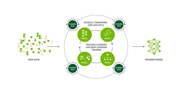
Figure 1. AI model training process
Training NGC models with Grid sessions, PyTorch Lightning, and NVIDIA NeMo
ASR is the task of transcribing spoken language to text and is a critical component of Speech to Text systems. When training ASR models, your goal is to generate text from a given audio input that minimizes the word error rate (WER) metric on human transcribed speech. The NGC catalog contains state-of-the-art pretrained models for ASR.
In the remainder of this post, we show you how to use Grid sessions, NVIDIA NeMo, and PyTorch Lightning to fine-tune these models on the AN4 dataset.
The AN4 dataset, also known as the Alphanumeric dataset, was collected and published by Carnegie Mellon University. It consists of recordings of people spelling out addresses, names, telephone numbers, and so on, one letter or number at a time, as well as their corresponding transcripts.
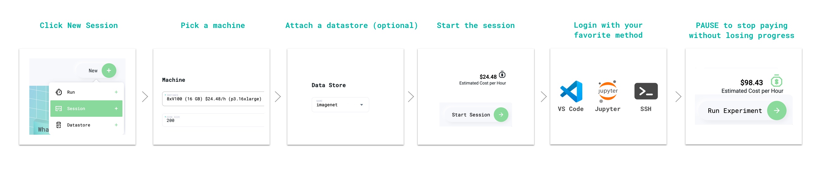
Step 1: Create a Grid session optimized for Lightning and pretrained NGC models
Grid sessions run on the same hardware that you need to scale while providing you with preconfigured environments to iterate the research phase of the machine learning process faster than before. Sessions are linked to GitHub, loaded with JupyterHub, and can be accessed through SSH and your IDE of choice without having to do any setup yourself.
With sessions, you pay only for the compute that you need to get a baseline operational, and then you can scale your work to the cloud with Grid runs. Grid sessions are optimized for PyTorch Lightning and models hosted on the NGC catalog. They even provide specialized Spot pricing.
For an in-depth walkthrough, see the Grid Session tour (requires a Grid.ai account).
Figure 2. Workflow to create a Grid session
Step 2: Clone the ASR demo repo and open the tutorial notebook
Now that you have a developer environment optimized for PyTorch Lightning, the next step is to clone the NGC-Lightning-Grid-Workshop repo.
You can do this directly from a terminal in your Grid Session with the following command:
After you’ve cloned the repo, you can open up the notebook to use to fine-tune the NGC hosted model with NeMo and PyTorch Lightning.
Step 3: Install NeMo ASR dependencies
First, install all the session dependencies. Run tools such as PyTorch Lightning and NeMo and process the AN4 dataset to do this. Run the first cell in the tutorial notebook, which runs the following bash commands to install the dependencies.
## Install dependencies
!pip install wget
!sudo apt-get install sox libsndfile1 ffmpeg -y
!pip install unidecode
!pip install matplotlib>=3.3.2
## Install NeMo
BRANCH = 'main'
!python -m pip install --user git+https://github.com/NVIDIA/NeMo.git@$BRANCH#egg=nemo_toolkit[all]
## Grab the config we'll use in this example
!mkdir configs
!wget -P configs/ https://raw.githubusercontent.com/NVIDIA/NeMo/$BRANCH/examples/asr/conf/config.yaml
Step 4: Convert and visualize the AN4 dataset
The AN4 dataset comes in raw Sof audio files, but most models process on mel spectrograms. Convert the Sof files to the Wav format so that you can use NeMo audio processing.
import librosa
import IPython.display as ipd
import glob
import os
import subprocess
import tarfile
import wget

# Download the dataset. This will take a few moments...
print("******")
if not os.path.exists(data_dir + '/an4_sphere.tar.gz'):
    an4_url = 'http://www.speech.cs.cmu.edu/databases/an4/an4_sphere.tar.gz'
    an4_path = wget.download(an4_url, data_dir)
    print(f"Dataset downloaded at: {an4_path}")
else:
    print("Tarfile already exists.")
    an4_path = data_dir + '/an4_sphere.tar.gz'

if not os.path.exists(data_dir + '/an4/'):
    # Untar and convert .sph to .wav (using sox)
    tar = tarfile.open(an4_path)
    tar.extractall(path=data_dir)

    print("Converting .sph to .wav...")
    sph_list = glob.glob(data_dir + '/an4/**/*.sph', recursive=True)
    for sph_path in sph_list:
        wav_path = sph_path[:-4] + '.wav'
        cmd = ["sox", sph_path, wav_path]
        subprocess.run(cmd)
print("Finished conversion.n******")
# Load and listen to the audio file
example_file = data_dir + '/an4/wav/an4_clstk/mgah/cen2-mgah-b.wav'
audio, sample_rate = librosa.load(example_file)
ipd.Audio(example_file, rate=sample_rate)
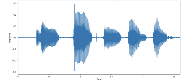
You can then visualize the audio example as images of the audio waveform. Figure 3 shows the activity in the waveform that corresponds to each letter in the audio, as your speaker here enunciates quite clearly!
Figure 3. Audio waveform of the sample example
Each spoken letter has a different “shape.” It’s interesting to note that the last two blobs look relatively similar, which is expected because they are both the letter N.
Spectrograms
Modeling audio is easier in the context of frequencies of sound over time. You can get a better representation than this raw sequence of 57,330 values. A spectrogram is a good way of visualizing how the strengths of various frequencies in the audio vary over time. It is obtained by breaking up the signal into smaller, usually overlapping chunks, and performing a short-time Fourier transform (STFT) on each.
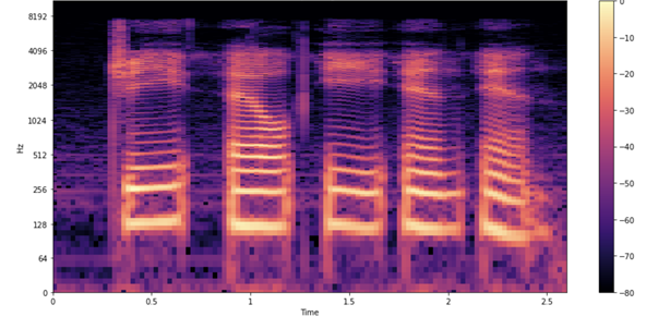
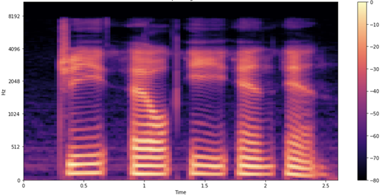
Figure 4 shows what the spectrogram of the sample looks like.
Figure 4. Audio spectrogram of the sample example
As in the earlier waveform, you see each letter being pronounced. How do you interpret these shapes and colors? Just as in the earlier waveform plot, you see time passing on the x-axis (all 2.6s of audio). However, now the y-axis represents different frequencies (on a log scale), and the color on the plot shows the strength of a frequency at a particular point in time.
Mel spectrograms
You’re still not done, as you can make one more potentially useful tweak by visualizing the data using the mel spectrogram. Change the frequency scale from linear (or logarithmic) to the mel scale, which better represents the pitches that are perceivable to the human ear. Mel spectrograms are intuitively useful for ASR. Because you are processing and transcribing human speech, mel spectrograms reduce background noise that can affect the model.
Figure 5. Mel spectrogram of the sample example
Step 5: Load and inference a pretrained QuartzNet model from NGC
Now that you’ve loaded and properly understood the AN4 dataset, look at how to use NGC to load an ASR model to be fine-tuned with PyTorch Lightning. NeMo’s ASR collection comes with many building blocks and even complete models that you can use for training and evaluation. Moreover, several models come with pretrained weights.
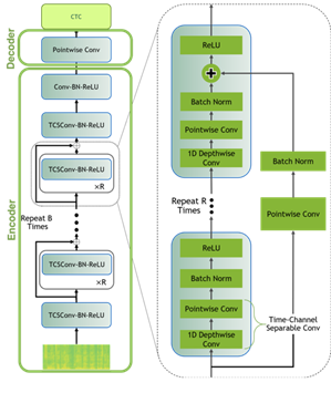
To model the data for this post, you use a Jasper architecture called QuartzNet from the NGC Model Hub. Jasper architecture consists of repeated block structures that uses 1D convolutions to model spectrogram data (Figure 6).
Figure 6. Jasper/QuartzNet model
QuartzNet is a better variant of Jasper with a key difference in that it uses time-channel separable 1D convolutions. This enables it to reduce the number of weights dramatically while keeping similar accuracy.
The following command downloads the pretrained QuartzNet15x5 model from the NGC catalog and instantiates it for you.
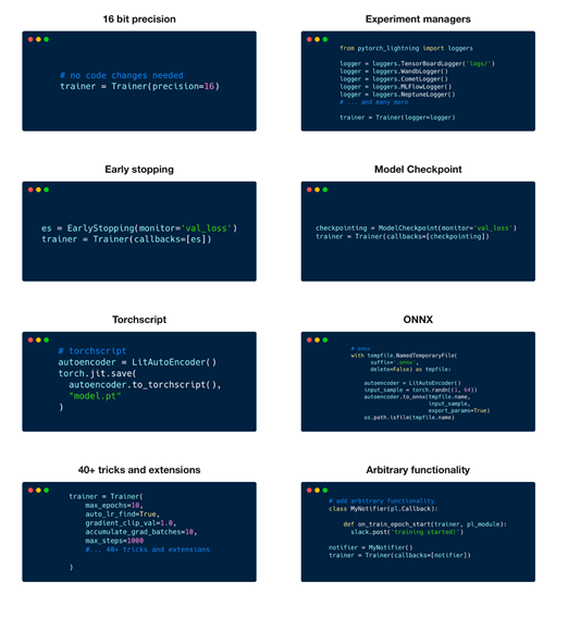
Because you are using this Lightning Trainer, you get some key advantages, such as model checkpointing and logging by default. You can also use 50+ best-practice tactics without needing to modify the model code, including multi-GPU training, model sharding, deep speed, quantization-aware training, early stopping, mixed precision, gradient clipping, and profiling.
Figure 7. Fine-tuning tactics
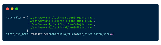
Step 7: Inference and deployment
Now that you have a baseline model, inference it.
Figure 9. Run inference
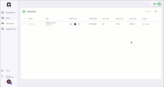
Step 8: Pause session
Now that you have trained the model, you can pause the session and all the files that you need are persisted.
Figure 9. Monitor Grid session
Paused sessions are free of charge and can be resumed as needed.
Conclusion
Now, you should have a better understanding of PyTorch Lightning, NGC, and Grid. You’ve fine-tuned your first NGC NeMo model and optimized it with Grid runs. We are excited to see what you do next with Grid and NGC.

 New research creates a low-cost and easy-to-use machine learning model to analyze streams of data from earth-imaging satellites.
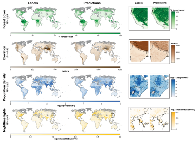


 NVIDIA Decision Support (NDS) is our adaptation of an industry-standard data science benchmark often used in the Apache Spark community. NDS consists of the same 105 SQL queries as the industry standard benchmark TPC-DS, but has modified parts for dataset generation and execution scripts.
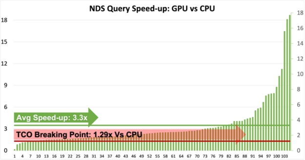
 PyTorch Lightning is a lightweight PyTorch wrapper for high-performance AI research. PyTorch code with Lightning enables seamless training on multiple-GPUs and uses best practices such as checkpointing, logging, sharding, and mixed precision. In this post, we walk you through building speech models with PyTorch Lightning on NVIDIA GPU-powered AWS instances managed by the Grid.ai platform.