DataBloom

This release offers Unreal Engine, NVIDIA RTX, and neural rendering advancements. 

This release offers Unreal Engine, NVIDIA RTX, and neural rendering advancements. 

Leading users and industry-standard benchmarks agree: NVIDIA H100 Tensor Core GPUs deliver the best AI performance, especially on the large language models (LLMs) powering generative AI. H100 GPUs set new records on all eight tests in the latest MLPerf training benchmarks released today, excelling on a new MLPerf test for generative AI. That excellence is Read article >

At the heart of the rapidly expanding set of AI-powered applications are powerful AI models. Before these models can be deployed, they must be trained through a…

At the heart of the rapidly expanding set of AI-powered applications are powerful AI models. Before these models can be deployed, they must be trained through a process that requires an immense amount of AI computing power. AI training is also an ongoing process, with models constantly retrained with new data to ensure high-quality results. Faster model training means that AI-powered applications can be deployed more quickly, speeding time to value. 

MLPerf benchmarks¹ are standardized and proven measures of AI performance across popular AI use cases. MLPerf Training v3.0 is the latest version of the AI training-focused suite of MLPerf tests, covering computer vision, language, and recommender systems, among others. The latest MLPerf Training v3.0 suite has been updated to incorporate a new large language model (LLM) test based on the GPT-3 175B model, representing generative AI. It also features an updated DLRM test with a substantially larger dataset to better represent modern AI-based recommenders. 

In MLPerf Training v3.0, the NVIDIA AI platform powered by the NVIDIA H100 Tensor Core GPU set new performance records, achieving both the highest performance on a per-accelerator basis and delivering the fastest time to train on every benchmark at scale. 

In addition, the full software stack used for MLPerf Training v3.0 is publicly available. Both NVIDIA submissions, as well as the joint submissions NVIDIA made with CoreWeave, were made in the available category of MLPerf. All NVIDIA submissions achieved similar or improved performance compared to NVIDIA H100 preview submissions in MLPerf Training v2.1. 

This post takes a closer look at the performance delivered by the NVIDIA AI platform and the H100 Tensor Core GPU in MLPerf Training v3.0. 

NVIDIA AI and H100 Tensor Core GPU deliver record results 

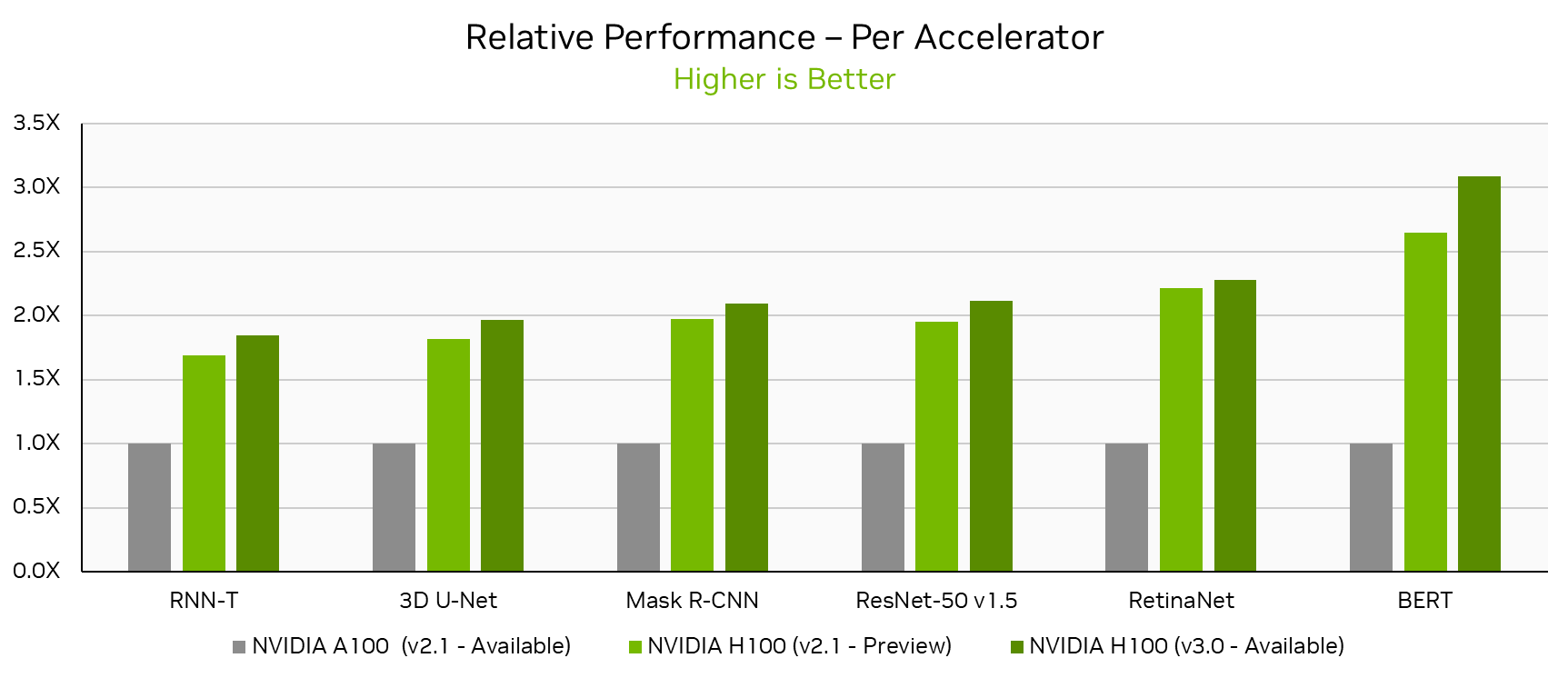
NVIDIA H100 Tensor Core GPUs, which made their MLPerf Training debut just 6 months ago, set new per-accelerator performance records across all MLPerf Training v3.0 workloads. Looking at the NVIDIA single-node DGX H100 results this round, performance increased by up to 17% in just 6 months on the same hardware through software improvements alone. Compared to the NVIDIA A100 Tensor Core GPU submission in MLPerf Training v2.1, the latest H100 submission delivered up to 3.1x more performance per accelerator. 

In this round, NVIDIA submitted results using the NVIDIA “Pre-Eos” AI supercomputer on up to 768 H100 GPUs. NVIDIA also made a joint submission with cloud service provider CoreWeave, using up to 3,584 H100 GPUs with the CoreWeave publicly available NVIDIA HGX H100 infrastructure.  

Across these submissions, the NVIDIA AI platform with H100 GPUs set new time-to-train records at scale across every workload, including the new LLM workload. 

Benchmark	Max Scale Records(minutes)
Large language model (GPT-3)	10.9
Natural language processing (BERT)	0.13 (8 seconds)
Recommendation (DLRMv2)	1.61
Object detection, heavyweight (Mask R-CNN)	1.47
Object detection, lightweight (RetinaNet)	1.51
Image classification (ResNet-50 v1.5)	0.18 (11 seconds)
Image segmentation (3D U-Net)	0.82 (49 seconds)
Speech recognition (RNN-T)	1.65

The following section details some of the software optimizations behind these results. 

NVIDIA software powering MLPerf results 

NVIDIA MLPerf Training v3.0 submissions included numerous optimizations that increased performance on existing and updated MLPerf Training workloads, and enabled excellent results on the new LLM test. 

Large language model 

The newly added LLM workload represents a state-of-the-art large language model with 175 billion parameters. Training this model requires full stack craftsmanship, as it stresses every part of an AI supercomputer, including compute, GPU memory bandwidth, and both internode and intranode interconnect capabilities.

In fact, the workload is so demanding that the smallest-scale NVIDIA submission on this workload used 512 of the latest H100 Tensor Core GPUs on the Pre-Eos system, achieving a time to train of 64.3 minutes. Scaling to 768 GPUs on the same Pre-Eos system reduced time-to-train to 44.8 minutes for near-linear scaling efficiency. 

NVIDIA and CoreWeave also made joint submissions on the LLM workload using CoreWeave’s NVIDIA HGX H100 infrastructure at several scales, including 768-GPU, 1,536-GPU, and 3,584-GPU submissions. The 768-GPU submission on CoreWeave’s HGX H100 infrastructure delivered nearly identical performance to the 768-GPU Pre-Eos submission, demonstrating that the NVIDIA AI platform delivers great performance in both on-premises and commercially available cloud instances.

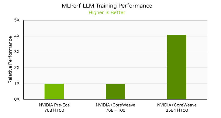
NVIDIA and CoreWeave also submitted LLM results on 3,584 GPUs, delivering a time to train of just 10.9 minutes. This is a more than 4x speedup compared to the 768-GPU submissions on H100, demonstrating 88% performance scaling efficiency even when moving from hundreds to thousands of H100 GPUs. 

The software stack used in the MLPerf LLM submission includes NVIDIA NeMo framework combined with the NVIDIA Transformer Engine library, as well as the intelligent use of 8-bit floating-point precision (FP8) on a per-layer basis on NVIDIA H100 GPUs.   

BERT

Compared to the prior round, NVIDIA improved per-accelerator H100 performance on the BERT NLP workload by 17%. And NVIDIA and CoreWeave submitted BERT results on up to 3,072 H100 GPUs to deliver a record-setting time to train of 0.134 minutes (a mere 8 seconds). 

In order to achieve this performance in publicly available NVIDIA software, the cuDNN library introduced FP8 I/O support in the fused Flash Attention used in the NVIDIA Transformer Engine library.  cuDNN fused Flash Attention also supports packed sequence format for Flash Attention I/O, enabling BERT to train at high efficiency without wasting compute on padding tokens. See the cuDNN Developer Guide for more details about cuDNN fused Flash Attention and its documentation.  

A summary of the key performance optimizations done in this round for BERT follows: 

Data preprocessing

When training models at very large scales, data preprocessing on the CPU may result in significant overhead. To minimize the performance impact of this preprocessing, we overlapped data preprocessing for the next iteration with the computations being performed in the current iteration, reducing iteration time by 3%. 

More performant random number generation 

In BERT Multi-Head Attention, the online random number generation for the dropout layer starts to become a bottleneck once operations in multi-head attention are fused into a single kernel. This is more pronounced as the Tensor Core throughput of recent NVIDIA GPU architectures has grown faster than the random number generation speed. 

To reduce the random number generation bottleneck, we introduced an optimization that uses a comparison of lower precision integer format (8-bit instead of 32-bit) in this MLPerf round, increasing random number generation throughput by 4x. In particular, instead of converting the random 128-bit integer that is produced by the random number generator to four 32-bit integers, we convert it to 16 8-bit integers. This optimization substantially reduces the overhead of random number generation in the multi-head attention block, and results in a 4% end-to-end performance improvement in the application for single-node submission. This optimization does not impact the accuracy or the output quality of the model. 

CUDA Graphs

In this submission, we enabled CUDA Graphs for large batch scenarios like training on eight GPUs, through graph-capture support in cuDNN fused Flash Attention and Transformer Engine library, which required carefully handling seed and offset variables of random number generator in multi-head attention.  

Furthermore, through optimizations we have reduced conversions between FP16 and FP8 formats and enabled new fused kernels. These optimizations combined boost single-node performance on BERT by 17% compared to the H100 preview submission in MLPerf Training v2.1. 

ResNet-50 v1.5

In MLPerf Training v3.0, NVIDIA and CoreWeave made submissions using up to 3,584 H100 Tensor Core GPUs, setting a new at-scale record of 0.183 minutes (just under 11 seconds). Additionally, H100 per-accelerator performance improved by 8.4% compared to the prior submission through software improvements.

In this round, key improvements on the ResNet-50 v1.5 workload include the following: 

Faster GroupBatchNorm with NVSHMEM

In this round, we implemented a faster GroupBatchNorm kernel using the NVIDIA NVSHMEM library and reducing inter-GPU communication latency by more than 5x. This new kernel is also able to make use of the high-bandwidth, inter-GPU NVIDIA NVLink interconnect to accelerate communication. This optimization resulted in an end-to-end speedup of 6% in the largest scale submission.

cuDNN kernels

The NVIDIA cuDNN team developed significantly improved convolution kernels that leverage the much faster Tensor Core throughput of the NVIDIA H100 GPU. These kernels led to 5% higher end-to-end performance in both single-node and efficient-scale submissions. 

RetinaNet

NVIDIA submitted results on RetinaNet using up to 768 NVIDIA H100 Tensor Core GPUs, achieving a new performance record for the benchmark of just 1.51 minutes. Per-accelerator performance was also enhanced compared to the prior submission. 

Optimizations of this round to achieve these results include:   

Support for FP32 Master Weights in the Optimizer

The NVIDIA RetinaNet submission in MLPerf Training v3.0 used PyTorch Automatic Mixed Precision (AMP) to leverage the higher throughput that the NVIDIA H100 GPU provides for lower precision data types, like FP16. 

However, as model parameters are still maintained in FP32, PyTorch AMP inserts dynamic type casting operations to convert between FP16 and FP32 data types while carrying out tensor operations in the lower precision. 

To avoid this overhead, the optimizer maintains a separate set of model parameters stored in FP32 called “master weights.” The model parameters can now be cast entirely to FP16, avoiding the insertion of dynamic type casting operations. The optimizer can update the master weights using the FP16 gradients obtained during the backward pass. This optimization boosted training performance by 10%. 

Data preprocessing

The NVIDIA RetinaNet submission uses the NVIDIA Data Loading Library (DALI), a portable, open-source library for decoding and augmenting images, videos, and speech to accelerate deep learning applications. 

In MLPerf Training v3.0, the NVIDIA submission used DALI for both data loading and preprocessing of variable-sized images in the dataset. By profiling our large-scale training runs using NVIDIA Nsight Systems, we observed that memory reallocation operations in DALI occur at different times for different processes in the training process, leading to delays in training iterations. 

Memory management operations in the DALI image decoder were one primary cause of jitter. These were removed by providing a hint to the largest image size in the dataset—an optimization that boosted performance by 10%. 

Optimizations in cuDNN

The cuDNN library has been updated with enhanced kernels that better use the NVIDIA H100 fourth-generation Tensor Cores. These kernels increased the performance of convolutions in our RetinaNet submission, particularly for the smaller-sized ones that are key to at-scale performance, leading to up to 7.5% higher training throughput compared to our prior submission. 

3D U-Net

NVIDIA submitted results on 432 NVIDIA H100 Tensor Core GPUs, achieving a new record for the benchmark of 0.82 minutes (49 seconds) to train. Per-accelerator performance on H100 also improved by 8.2% compared to the prior round. 

To achieve excellent performance at scale, a faster GroupBatchNorm kernel was one key optimization. 

In our largest scale 3D U-Net submission, the instance normalization operation in the neural network needs to perform a reduction of the tensor mean and variance across four GPUs. By using a faster GroupBatchNorm kernel to implement instance normalization, we delivered a 1.5% performance increase. 

Mask R-CNN

This round, NVIDIA submitted results on Mask R-CNN using up to 384 H100 GPUs, achieving a new record time to train of 1.47 minutes. Per-accelerator performance also improved by 6.1% compared to the previous submission through software optimizations. 

Optimizations this round focused on reducing CPU bottlenecks to ensure that the capabilities of the powerful H100 GPUs were better used. 

Faster evaluation

The evaluation process computes the score after inference results have been gathered on a single rank. Since the H100 GPU is able to train significantly faster than the prior-generation A100 GPU, evaluation became a significant performance bottleneck. 

In this round, each individual inference result is encoded as JSON (corresponding to a single prediction for each image) before gathering the results on a single rank. After the results were gathered, JSON strings for collections of inference results were formed by concatenating strings from the initial JSON encoding, rather than by decoding and encoding inference results as they passed through the scoring logic. This approach is substantially faster than encoding and decoding and yields a doubling in evaluation speed. 

Faster annotations

In previous rounds, annotations—which contain target information for each sample—were loaded from a very large JSON file, a process that took up to 5 seconds. By storing annotations as serialized tensors and loading them, we reduced startup time by more than 80%. 

Before annotations can be used for training, they must undergo transformations. Instead of performing these transformations independently for each image, we performed all transformations with a single global kernel as all images undergo the same transformations. This kernel is called once during load and is repeated at the beginning of each epoch. 

This optimization reduced the amount of CPU work by nearly 20%. As Mask R-CNN was CPU-limited, training performance increased by almost 20%. 

More CUDA graphs

In prior rounds, we CUDA-graphed everything except for loss calculations. We observed that loss calculations accounted for more than 40% of total step time, due to the loss calculation code being CPU bound. By CUDA-graphing the entire model, we improved training throughput by more than 30%. 

DLRM_DCNv2 

DLRM_DCNv2 is a new benchmark in MLPerf Training v3.0. It replaces the previous DLRM benchmark, with the following updates:

1. Multi-hot dataset: The previous DLRM benchmark used a one-hot Criteo dataset. To better represent real-world use and application of recommenders, DLRM_DCNv2 adopts a multi-hot dataset. A multi-hot dataset has been synthesized from the original Criteo one-hot dataset for this purpose.
2. Cross layer: The cross layer proposed in the paper DCN V2: Improved Deep and Cross Network and Practical Lessons for Web-scale Learning to Rank Systems is introduced for DLRM_DCNv2.
3. Adagrad optimizer: The SGD optimizer used in DLRM is replaced with Adagrad optimizer in DLRM_DCNv2, as Adagrad is more commonly used in real-life recommenders.   

Our submission uses the embedding collection in NVIDIA Merlin HugeCTR, which supports many sharding strategies and horizontally fuses embedding operations associated with different embedding shards to deliver excellent performance.  

For scale-out training, we employed a hierarchical embedding strategy to leverage the hierarchical nature of the network fabric. This approach resulted in the following benefits:

1. Embedding vectors in the same node are reduced by first leveraging NVIDIA NVLink connections to reduce the number of bytes needed to be transferred through the InfiniBand networking connecting GPUs between nodes.
2. The reduced embedding vectors are then placed on GPUs that share the same InfiniBand rails as the destination GPU, minimizing transmission latency in rail-optimized systems.

The NVIDIA submission employed a module called input distributor in the embedding collection for performance and flexibility. This module converts the data-parallel input from the data reader to the model-parallel input needed by the embedding operations. To reduce the amount of traffic associated with the input distribution, category filtering is employed to only transmit the categories needed by each GPU. Furthermore, input data is prefetched and distributed to overlap the input distribution of the next iteration with the current iteration, thereby boosting training throughput.

MLPerf Training v3.0 takeaways

The NVIDIA AI platform delivered record-setting performance in MLPerf Training v3.0, highlighting the exceptional capabilities of the NVIDIA H100 GPU and the NVIDIA AI platform for the full breadth of workloads—from training mature networks like ResNet-50 and BERT to training cutting-edge LLMs like GPT-3 175B. The NVIDIA joint submission with CoreWeave using their publicly available NVIDIA HGX H100 infrastructure showcased that the NVIDIA platform and the H100 GPU deliver great performance at very large scale on publicly-available cloud infrastructure. 

The NVIDIA platform delivers the highest performance, greatest versatility, and is available everywhere. All software used for NVIDIA MLPerf submissions is available from the MLPerf repository, so you can reproduce these results. 

¹The MLPerf name and logo are trademarks of MLCommons Association in the United States and other countries. All rights reserved. Unauthorized use strictly prohibited. See www.mlcommons.org for more information.

NVIDIA and Snowflake announced a new partnership bringing accelerated computing to the Data Cloud with the new Snowpark Container Services (private preview), a…

NVIDIA and Snowflake announced a new partnership bringing accelerated computing to the Data Cloud with the new Snowpark Container Services (private preview), a runtime for developers to manage and deploy containerized workloads. By integrating the capabilities of GPUs and AI into the Snowflake platform, customers can enhance ML performance and efficiently fine-tune LLMs. They achieve this by leveraging the NVIDIA AI Enterprise software suite on the secure and governed Snowflake platform. With this collaboration, customers can develop cost-effective AI-powered applications using their valuable data.

About NVIDIA AI Enterprise 

As AI initiatives progress, the need for a trusted, scalable support model for enterprises becomes vital to making sure AI projects stay on track. To support building AI applications, NVIDIA AI Enterprise includes the software to streamline the end-to-end AI pipeline, from data prep, to model training, to simulation, and deploying at scale.

NVIDIA AI Enterprise is the software layer of the NVIDIA AI platform and includes:

• Optimizations to run on accelerated infrastructure for performance, productivity, and cost savings. 
• Enterprise-grade support, security, and API stability. 
• AI workflows and pretrained models to speed time to production.
• Certifications to deploy everywhere—cloud, data center, and edge. 

Enable AI workflows directly on Snowflake Data Cloud

​​​Data is the fuel for generative AI—and the data fueling enterprise AI use cases lives in Snowflake. With the NVIDIA AI platform now available on Snowpark Container Services, customers can put their data to work without sacrificing security, performance, or ease of use. 

Using the NVIDIA AI Enterprise accelerated infrastructure and computing libraries through Snowpark Container Services, developers and data scientists can build accelerated AI workflows with ease. 

With Snowpark, enterprises securely deploy and process their Python code used for AI and ML. Developers can also expand accelerated ML workloads and run sophisticated AI models such as LLMs where their data is already stored. ​​This reduces potential security risks and latency ‌when moving large amounts of data.

The following workflow shows how a data scientist can implement each stage, from data processing to real-time inferencing, as part of the new partnership. The technologies outlined in this workflow and example use case, including NVIDIA RAPIDS, NVIDIA Merlin, NVIDIA TensorRT, and NVIDIA Triton are all included with NVIDIA AI Enterprise and available on Snowpark Container Services. 

Example use case: training a recommender model

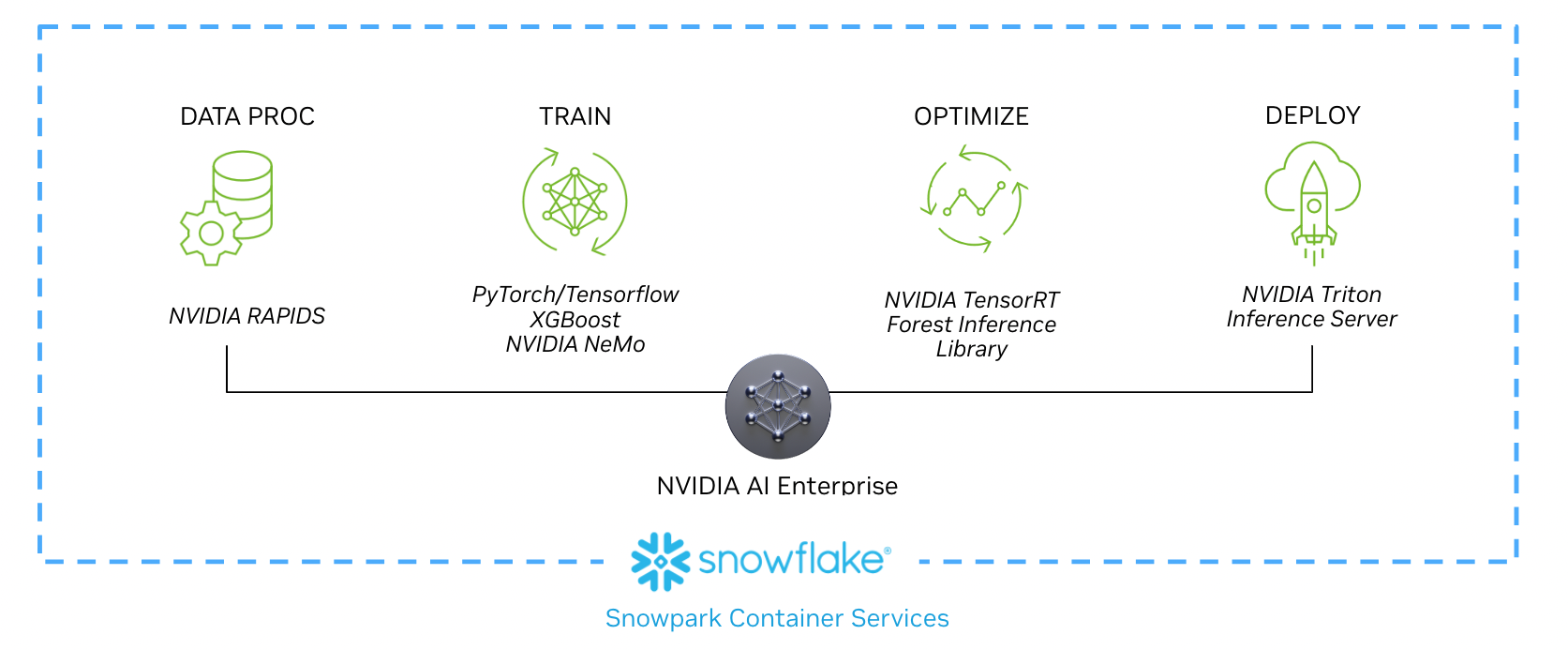
Session-based recommender systems are becoming increasingly important in content-rich applications aiming to provide more relevant next-item predictions. Training these models starts by loading data and conducting initial SQL and DataFrame preprocessing using the Snowpark Python library. 

Customers can use NVIDIA RAPIDS, Merlin, and other AI frameworks in a Jupyter Notebook running in Snowpark Container Services to augment data processing and train models. 

NVTabular, part of Merlin, is an accelerated feature engineering library designed to generate key features needed in recommender systems model training. After the data is prepared using NVTabular, additional accelerated computing libraries in Merlin begin training the AI workflow.

The task of training a model on very large datasets can be time-consuming. During training, the dataset is often copied in and out of memory in chunks while compute cores process it. Training a model using a GPU provides higher throughput and faster model training because they include high-bandwidth memory and make use of an increased number of compute cores for parallel processing.

Operating on Snowpark Container Services results in a 20X speedup during the training of a predictive model with accelerated compute. This boosts the productivity of data scientists during model creation and reduces the overall TCO by doing more, in less time. 

After training, the model is tested for accuracy with sample test data. The workflow then optimizes and retrains the model as needed. Finally, it publishes the newly trained model to a registry such as the Snowpark Model Registry (private preview).

After training, NVIDIA AI Enterprise provides TensorRT, optimizing for accelerated computing. At the final stage in the workflow, the model deploys and begins performing inference tasks. Running inside a Triton Inference server, it consumes data in real time and provides insights. 

Request access to get started

Snowflake customers can request access to the technical preview of the Snowpark Container Services from their account team. Customers are also eligible for a free NVIDIA AI Enterprise 90-day evaluation license to make sure they have access to the full stack of NVIDIA AI software.  

Learn more about NVIDIA AI Enterprise.

Learn more about Snowpark Container Services.

Editor’s note: This post is a part of our Meet the Omnivore series, which features individual creators and developers who accelerate 3D workflows and create virtual worlds using NVIDIA Omniverse, a development platform built on Universal Scene Description, aka OpenUSD. As augmented reality (AR) becomes more prominent and accessible across the globe, Kiryl Sidarchuk is Read article >

Single-cell sequencing has become one of the most prominent technologies used in biomedical research. Its ability to decipher changes in the transcriptome and…

Single-cell sequencing has become one of the most prominent technologies used in biomedical research. Its ability to decipher changes in the transcriptome and epigenome on a cell level has enabled researchers to gain valuable new insights. As a result, single-cell experiments have grown in size and complexity by a factor of over 100, with experiments involving more than 1 million cells becoming increasingly common. 

However, the resulting data must be analyzed in a highly iterative process. It is crucial that fast algorithms are used for these iterative steps to enable quick turnaround times.

For more consistent single-cell analysis using Python, developers at scverse have worked toward building an entire ecosystem to help researchers perform analyses. At the core of this ecosystem lies a data structure that maintains annotations of various transformations throughout the data processing pipeline during single-cell analysis. 

AnnData, a Python package for handling annotated data matrices in memory and on disk, is the core structure used in the Scanpy library, which is the main single-cell analysis suite within the scverse ecosystem. Scanpy builds on top of other libraries common to the PyData ecosystem—such as NumPy, SciPy, Numba, and Scikit-learn—for just about all of the typical analysis steps. 

However, Scanpy algorithms are mostly CPU-based and slow down significantly with larger experiments. The highly iterative nature of the single-cell analysis process only compounds this problem. 

GPUs for single-cell analysis

General feasibility of running downstream single-cell RNA sequencing (scRNA-seq) analysis on the GPU with RAPIDS and Scanpy has been shown in Accelerating Single-Cell Genomic Analysis with GPUs. This work resulted in the rapids-single-cell-examples GitHub repo, which contains a series of example notebooks written by the RAPIDS and NVIDIA Parabricks teams. RAPIDS is an open-source suite of libraries for GPU-accelerated data science with Python. Parabricks is a free suite of GPU-accelerated, industry-standard genomic analysis tools based on deep learning.

While these example notebooks demonstrate a few typical single-cell RNA workflows on the GPU, they were never intended for daily use nor as a GPU-accelerated replacement for libraries like Scanpy. 

Drawing inspiration from prior work on rapids-single-cell-examples is an emerging library called rapids-singlecell, a GPU-accelerated tool for scRNA analysis. This tool aims to be a daily drivable single-cell analysis suite that is compatible with the scverse ecosystem. It uses RAPIDS and CuPy to provide GPU-accelerated functions that are near-drop-in replacements for the corresponding functions in Scanpy.

On average, users can expect performance to increase between 10x and 20x by using rapids-singlecell. For more details, see Accelerating Single Cell Genomic Analysis Using RAPIDS.

Faster single-cell analysis using RAPIDS

rapids-singlecell follows a similar usability model as the scverse Python libraries. It is also written in Python but puts many of the performance-critical pieces on the GPU, hiding all of the complexities that are normally associated with writing CUDA applications (the language typically used to write accelerated algorithms for NVIDIA GPUs). 

rapids-singlecell consists of five categories, which are described in the sections that follow. Each category accelerates a different piece of the typical single cell analysis workflow.

For more information, including the various APIs offered by rapids-singlecell, see the rapids-singlecell documentation. 

cunnData

The AnnData, or annotated data object, is a widely used data structure for handling single-cell RNA sequencing data. As shown in Figure 1, it consists of several attributes, including a count matrix attribute, X, which represents the expression levels of genes in each cell. AnnData objects also contain annotation dataframes for cells (.obs attribute) and genes (.var attribute), which store additional information such as cell type and gene names.

In contrast, cunnData (Figure 1) is a minimized and lightweight version of the AnnData object for the GPU that replaces the scverse standard for preprocessing. Instead of storing the count matrix .X on the CPU, cunnData stores it on the GPU as CuPy sparse matrices. This makes it faster and more efficient to perform computations on the count matrix.

cunnData also includes additional features, such as the ability to store different versions of the count matrix, such as raw integer counts, in .Layers. Unlike AnnData, which stores .Layers in Host (CPU) memory, cunnData also stores .Layers on the GPU, reducing the need to copy data from the host to GPU memory and enabling accelerated computations.

cunnData supports unstructured annotations in the .uns attribute, as well as multidimensional annotations of cells and genes in the .obsm and .varm attributes, which are stored in the host memory. These annotations enable users to include additional information about their data, such as spatial coordinates or principal component analysis (PCA) embeddings.

Similarly, cunnData supports slicing like AnnData. These slices, however, are always full copies of the original data, as opposed to views. Overall, cunnData enables a faster approach to preprocessing scRNA-seq data compared to the more feature-rich CPU-bound AnnData object.

The Python snippet below demonstrates the conversion of an AnnData object (a standard data structure for handling single-cell RNA sequencing data) into a cunnData object.

import scanpy as sc
import rapids_singlecell as rsc
adata = sc.read("PATH TO DATASET")
cudata = rsc.cunnData.cunnData(adata=adata) 

Preprocessing

The preprocessing functions are stored in cunnData_funcs, which provides accelerated alternatives to the Scanpy preprocessing functions. These functions work on the cunnData object and use RAPIDS cuML and CuPy to dramatically accelerate Scanpy functions based on Scikit-learn, Numpy and SciPy.

Filtering cells and genes can be accomplished with filter_cells and filter_genes functions, respectively. Quality control is handled with the calculate_qc_metrics function.

# Basic QC rapids-singlecell
rsc.pp.flag_gene_family(cudata,gene_family_name="MT", gene_family_prefix="mt-")
rsc.pp.calculate_qc_metrics(cudata,qc_vars=["MT"])
cudata = cudata[cudata.obs["n_genes_by_counts"] > 500]
cudata = cudata[cudata.obs["pct_counts_MT"] 



To normalize your data, cunnData_funcs provides GPU alternatives to the normalize_total, log1p, and the recently introduced normalize_pearson_residuals functions from Scanpy. Annotating highly variable genes is accelerated for all flavors supported in Scanpy (including seurat, cellranger, seurat_v3, pearson_residuals), as well as poisson_gene_selection, which is adapted from scvi-tools.



# log normalization and highly variable gene selection
cudata.layers["counts"] = cudata.X.copy()
rsc.pp.normalize_total(cudata,target_sum=1e4)
rsc.pp.log1p(cudata)
rsc.pp.highly_variable_genes(cudata,n_top_genes=5000,flavor="seurat_v3",layer = "counts")
cudata = cudata[:,cudata.var["highly_variable"]==True]

The regress_out function, used to remove unwanted sources of variation, is accelerated with the cuML linear regression estimator. It also supports multitarget regression, which was introduced in cuML in version 22.12, while staying backwards compatible with prior versions. 
Principal component analysis wraps cuML PCA, Truncated SVD, and Incremental PCA to give you the same options offered by Scanpy. With the PCA version in cunnData_funcs, you can choose which layer you want to use for the analysis, an additional feature not currently supported by the scanpy PCA function.
# Regression, scaling and PCA
rsc.pp.regress_out(cudata,keys=["total_counts", "pct_counts_MT"])
rsc.pp.scale(cudata,max_value=10)
rsc.pp.pca(cudata, n_comps = 100)

sc.pl.pca_variance_ratio(cudata, log=True,n_pcs=100)

cunndata_funcs can accelerate preprocessing by a factor of 10 to 20x (Tables 1-3). After preprocessing, the cunnData object is transformed into an AnnData object.
adata_preprocessed = cudata.to_AnnData()
Tools
scanpy_gpu provides functions that work on the AnnData object, with the goal of providing accelerated functions. To keep the syntax as close as possible between Scanpy and rapids-singlecell, metadata is also written to the .uns attribute. This attribute is useful for storing trained parameters such as the variance ratio, which is computed during the PCA computation. scanpy_gpu provides a PCA function for the AnnData object equivalent to cunnData_funcs.
Scanpy already includes support for computing UMAP and nearest neighbors on the GPU using cuML. scanpy_gpu extends Scanpy GPU support by adding more algorithms, such as accelerated graph-based clustering using Leiden and Louvain from cuGraph, as well as the Force Atlas 2 algorithm for visually laying out graph data. scanpy_gpu also uses PCA and kernel density estimation (KDE)  from cuML and diffusion maps are computed using the CuPy library in a similar manner to how Scanpy uses SciPy and Numpy for scientific computing. 
For batch correction, scanpy_gpu provides a GPU port of Harmony Integration, called harmony_gpu. PyMDE (minimum distortion embedding), a function that enables embedding single-cell data while jointly learning the graph and the low-dimensional representation in a probabilistic manner, has also been adapted from scvi-tools.
The near-drop-in replacement nature of rapids-singlecell relies on Scanpy for visualization. It is intuitive to use Scanpy for plotting directly within the scverse framework.
Decoupler
The decoupler tool uses a unified framework to implement several different statistical methods with a focus on biological activity. (Cellular, molecular, and physiological processes in living organisms, for example, gene sets and transcription factors activity.) decoupler_gpu re-implements and accelerates the weighted sum (run_wsum) and multivariate linear model (run_mlm) methods. The GPU port in rapids-singlecell uses the same nets/models as decoupler. Table 1 shows a performance increase of up to 37x for wsum.
Squidpy developments
rapids-singlecell is continually expanding with new accelerated functions for the scverse ecosystem. Comprehensive tests have been added to the library to ensure the correctness and reliability of the code. Squidpy enables detailed analysis and visualization of spatial molecular data. It facilitates understanding of complex cell interactions and spatial patterns, greatly contributing to the expansion of the scverse ecosystem. 
Some functions have been accelerated with rapids-singlecell. Spatial auto-correlation with Moran’s I and Geary’s C promises a performance increase of up to 100x. The ligand-receptor (ligrec) interaction analysis in Squidpy has also been optimized and accelerated, resulting in a performance increase of more than 10x.
Benchmarks
Our benchmark results show that using GPU acceleration with the rapids-singlecell package and the decoupler functions can significantly improve the performance of scRNA-seq analysis. 
For example, running a sample rapids-singlecell notebook with about 90 K cells end-to-end on a server node with two AMD Epyc Milan 7543, 500 GB memory, and an NVIDIA A100 80 GB GPU was completed in just 51 seconds using the rapids-singlecell package, compared to 1,106 seconds with the traditional scanpy CPU workflow. 
Similarly, the decoupler functions also demonstrated significant speed improvements, with the mlm function running in just 12 seconds on the GPU compared to 83 seconds on the CPU, and the wsum method completing in just 26 seconds on the GPU compared to 16 minutes and 10 seconds on the CPU. 
Overall, these results demonstrate the potential for GPU acceleration to make scRNA-seq analysis faster and more efficient. These benchmark results are summarized in Table 1.




Function
CPU 
GPU
Speedup


Whole notebook(excluding decoupler functions)
1,106 s  (18.5 min)
51 s
21x


Preprocessing
74 s 
8 s
9x


Regress out
27 s
1.6 s
16x


PCA
35 s
0.7 s
50x


HVG (Seurat v3)
3.2 s
0.4 s
8x


Harmony
417 s
18 s
23x


Neighbors
22 s
5.1 s
4.3x


UMAP
36 s
0.4 s
90x


TSNE
133 s
2.4 s
55x


Louvain
17 s
0.6 s
28x


Leiden
14 s
0.2 s
70x


Logistic regression
58 s
3.7 s
15x


Draw graph (FA2)
256 s
0.3 s
850x


run_mlm (DoRothEA)
83 s
12 s
7x


Run_wsum (PROGENy)
970 s (16 min)
26 s
37x



In addition to the previous benchmark results, running a sample rapids-singlecell notebook with 500 K cells on the server node takes about 2 minutes when using rapids-singlecell. The same analysis takes about 41 minutes on the CPU.
Furthermore, using pearson_residuals for highly variable gene selection and normalization can also be accelerated using GPUs, providing additional speed improvements in scRNA-seq analysis. These benchmark results are summarized in Table 2.
rapids-singlecell is not only capable of accelerating single-cell data analysis on high-end server nodes, but also on consumer-grade hardware. Running the same notebook end-to-end with 50,000 cells on a desktop system with an AMD 5950x CPU, 64 GB memory, and an NVIDIA RTX 3090 GPU, takes around 5 minutes using rapids-singlecell. Although the system was using the RAPIDS Memory Manager (RMM) and unified memory to oversubscribe the GPUs memory, it saw a significant speedup compared to the CPU server. These benchmark results are summarized in Table 2.




Function
CPU
GPU (A100)
GPU (3090)
Speedup


Whole notebook(excluding PR functions)
2,460 s (41 min)
110 s
290 s
22x


Preprocessing 
305 s 
28 s
169 s
10x


HVG (Seurat v3)
48 s
1.5 s
13 s
32x


Regress out
104 s
5.1 s
16 s
20x


scale
8.4 s
1.3 s
5 s
6.4x


PCA
86 s
3.7 s
35 s
23x


Neighbors
74 s
17.1 s
18.3 s
4.3x


UMAP
281 s (4.6 min)
6.7 s
7.6 s
60x


TSNE
786 s (13 min)
10 s
12.9 s
105x


Louvain
283 s (4.5 min)
4.5 s
5.7 s
62x


Leiden
282 s (4.5 min)
0.6 s
0.9 s
470x


Logistic regression
452 s (7.5 min)
33 s
63 s
13x


Diffusion map
30 s
0.75 s
1.3 s
40x


HVG (PR)
104 s 
2.1 s
15.6 s
50x


Normalize (PR)
22 s
0.3 s
1 s
73x



Running the same sample notebook (Table 1) with about 90 K cells end-to-end on the desktop system takes only 48 seconds when using rapids-singlecell. In comparison, the traditional scanpy CPU workflow takes 774 seconds. The accelerated decoupler functions also demonstrate significant speed improvements on consumer-grade hardware. These benchmark results are summarized in Table 3.




Function
CPU 
GPU
Speedup


Whole notebook(excluding decoupler functions)
774 s (13 min)
48 s
16x


Preprocessing
114 s 
6 s
19x


Regress out
62 s
1.6 s
39x


PCA
42 s
0.7 s
60x


HVG (Seurat v3)
2.7s
0.4 s
6.7x


Harmony
175 s
21.7 s
8x


Neighbors
14.9 s
4.6 s
3.2x


UMAP
31 s
0.3 s
103x


TSNE
95 s
1.4 s
68x


Louvain
9.3 s
0.5 s
18x


Leiden
13.2 s
0.1 s
130x


Logistic regression
76 s
3.75 s
20x


Draw graph (FA2)
191 s
0.23 s
830x


run_mlm (DoRothEA)
55 s
12 s
4.5x


Run_wsum (PROGENy)
690 s (11.5 min)
28 s
26x



Installation 
There are multiple methods for installing rapids-singlecell. The easiest method is to use one of the provided yaml files provided within the GitHub repository. These set up the entire environment with everything needed for running the example notebooks.
conda create -f conda/rsc_rapids_23.02.yml

You can also install rapids-singlecell from PyPI into a Conda environment and install RAPIDS from Conda. The default installer does not include RAPIDS or CuPy. Scanpy is also excluded because it is technically not necessary.
pip install rapids-singlecell


Finally, you can install the entire library, including the RAPDIS dependencies, from PyPI using the new experimental PyPI packages from RAPIDS. However, this method of installation requires the user to properly set up CUDA so that it can be found by RAPIDS and CuPy. 
To do this, you can use the following command:
pip install 'rapids-singlecell[rapids]’ --extra-index-url=https://pypi.nvidia.com


Conclusion
With the rapids-singlecell library, it is possible to run the complete analysis of 500 K cells in less time than it takes a CPU to compute only its UMAP embedding. Therefore, it enables a much faster iterative process in single-cell data analysis stages. 
rapids-singlecell also enables the bioinformatician to analyze the data with a physician or biologist in real time, leading to better collaboration and interpretation of the data. In our experience, it is possible to analyze 200 K cells without any issues, even on a consumer-class 3090 series graphics card. Even better, RMM enables the GPU memory to be oversubscribed and spilled to the main memory, enabling scales well over 500 K cells.
With the datacenter-class NVIDIA A100 80 GB GPU, you can analyze matrices containing as many as 231-1 (approximately 2.15 billion) non-zero counts. (Note that this is the current limit imposed by the CuPy 32-bit integer-based indexing for sparse matrix calculations.) This powerful capability enables users to analyze datasets with over 1 million cells. 
The upwards of 20x speedup that rapids-singlecell provides enables researchers to focus more on analyzing and interpreting their single-cell data, rather than waiting for lengthy computational processes. In the true spirit of RAPIDS, this ultimately enhances productivity and fosters new insights into cellular biology that were not possible before.

		

While generative AI is a relatively new household term, drug discovery company Insilico Medicine has been using it for years to develop new therapies for debilitating diseases. The company’s early bet on deep learning is bearing fruit — a drug candidate discovered using its AI platform is now entering Phase 2 clinical trials to treat Read article >

Snowflake, the Data Cloud Company, and NVIDIA today announced at Snowflake Summit 2023 that they are partnering to provide businesses of all sizes with an accelerated path to create customized generative AI applications using their own proprietary data, all securely within the Snowflake Data Cloud.

As data generation continues to increase, linear performance scaling has become an absolute requirement for scale-out storage. Storage networks are like car…

As data generation continues to increase, linear performance scaling has become an absolute requirement for scale-out storage. Storage networks are like car roadway systems: if the road is not built for speed, the potential speed of a car does not matter. Even a Ferrari is slow on an unpaved dirt road full of obstacles.

Scale-out storage performance can be hindered by the Ethernet fabric that connects the storage nodes. NVIDIA accelerated Ethernet can remove performance bottlenecks, enabling maximum storage performance for applications in general, and AI/ML in particular.

Scale-out storage requires a strong network

Every second, 54,000 pictures are taken worldwide. By the time you read this, that number will be even higher. No matter what your business is, chances are you have massive amounts of data that must be stored and analyzed, with the amount growing every day. 

The old scale-up approach of using ever-larger storage filers has been replaced with a scale-out approach to deliver storage that scales linearly in both capacity and performance.

With scale-out storage, or distributed storage, several smaller nodes are configured and connected to act as one logical unit. A single file or object can be spread across many nodes. 

As more scale is needed, additional storage nodes are easily added to increase both storage capacity and performance. This applies to both a traditional enterprise storage vendor solution, or a software-defined solution, with the software and hardware sourced independently. 

Distributed storage enables flexible scaling and cost efficiency, but requires a high-performance network to connect the storage nodes. Many data center switches are ill-suited to the unique traffic characteristics of storage, and in fact can cripple the performance of scale-out storage solutions.  

How storage traffic is different from traditional traffic

For many use cases, network traffic is consistent and homogeneous, and traditional Ethernet suffices. However, traffic generated by storage devices may cause the issues detailed below.

Network stress 

Current storage solutions benefit from faster SSDs and storage interfaces, such as NVMe and PCIe Gen 4 (soon PCIe Gen 5), that are designed to provide higher performance. 

Congestion 

When the storage fabric is saturated, network congestion becomes inevitable, just like roadway congestion when too much traffic is on the highway. Network congestion is particularly problematic for scale-out storage because each storage node is expected to offer fast data delivery. But when congestion occurs, many data center switches have a fairness problem, where some nodes will be slowed much more than others. A single file or object is usually spread across many nodes, so anything that slows a single node effectively slows the whole cluster.

Bursty traffic

Most storage workloads are bursty, generating intense data transfers and repeatedly requiring large amounts of bandwidth for short periods. When that happens, the network switch must use its buffer to absorb the burst until the transient burst is over, thus preventing packet loss. Otherwise, that packet loss will require data retransmissions, significantly deteriorating application performance.

Storage jumbo frames 

Traditional data center network traffic uses a maximum packet size (MTU) of 1.5 KB. Scale-out storage nodes perform better when they can use 9 KB “jumbo frames,” which increase throughput while reducing ‌CPU processing overhead. Many data center switches built with commodity switch ASICs perform poorly or unpredictably with jumbo frames.

Low latency 

One of the ways storage IOPs have improved is through the orders-of-magnitude latency reduction for the read/write operations in flash-based media. ‌However, those costly performance improvements can be lost when the network introduces high latency—especially due to excessive buffering.

Both training and inference require adequate amounts of data with high-speed access, to make sure that GPU processors are fed quickly enough to keep them fully engaged. During training, WRITE operations are performed by all nodes to improve model accuracy. This results in a burst, making it imperative for switches to handle congestion effectively. Finally, lower storage latency enables GPUs to handle compute tasks more efficiently.

Why ASICs are suboptimal for storage traffic 

Most data center switches are built using commodity switch ASICs that were cost-optimized for traditional data traffic patterns and packet sizes. To keep costs low while achieving their bandwidth targets, Ethernet switch chip vendors compromised fairness by using a split buffer architecture.

Every switch has a buffer to absorb traffic bursts and prevent packet loss when congestion occurs. The common approach is to have a buffer that is shared across many ports. However, not all shared buffers are the same—there are different buffer architectures.

Commodity switches do not have a fully shared buffer—they use either an ingress-shared buffer, or an egress-shared buffer. 

With an ingress-shared buffer, there is a static mapping between a group of incoming ports and a specific memory slice. These ports can use only the memory in that assigned slice and not the whole buffer, not even if the rest of the buffer is available and no one is using it. 

With an egress-shared buffer, the mapping is between a group of outgoing ports and a specific buffer memory slice. Again, each group of egress ports can only use its assigned buffer slice, not the whole buffer.

With these two architectures, flows that stay within the same memory slice do not behave like flows that travel between memory slices. If many flows use ports with the same buffer, those ports will experience higher latency and lower throughput, while traffic using other slices of the buffer will enjoy higher performance. 

The storage performance depends on which ports the storage traffic (and other traffic) is using and how busy are the buffer slices for those ports. This is why switches that use split buffers often experience issues related to fairness, predictability, and microburst absorption.

Why deep-buffer switches are suboptimized for storage 

Deep-buffer switches usually refer to a switch that offers much more buffering (GBs rather than MBs). Deep-buffer switches are often promoted for use as routers, because they can absorb and hold large traffic bursts if there is a mismatch in network speeds or an incast situation. 

But in most data center applications, including scale-out storage, the deep-buffer switches negatively impact performance for the following reasons:

Job completion time 

With parallel file systems, the storage node with the slowest response dictates the time required to fetch a file. Unlike commodity switch ASICs that have a sliced on-chip buffer, deep-buffer switches have both on-chip and off-chip buffers, and they all are sliced, not fully shared, buffers. 

Think of how many ways flows can go before they leave the switch. They can stay within one on-chip memory slice (fastest), travel between on-chip memory slices (slower), or travel between on-chip and off-chip memory slices (very slow). 

All these flows will behave differently, and hence will cause fairness and predictability issues for storage traffic. Because these issues slow down one or more nodes, they adversely impact job completion time and slow down the whole distributed storage cluster.

Latency

The larger the switch buffer, the longer the queue each packet must go through and the greater the latency. The tested average port-to-port latency of a deep-buffer switch is more than 500 microseconds. Compared to a fully shared buffer switch from the same generation, NVIDIA Spectrum 1 latency is just 0.3 microseconds. It requires nanoseconds rather than microseconds to switch/route a packet. 

Deep-buffer latency is 1,000x higher. You may be wondering, is this just happening when congestion occurs? No. Under congestion, deep-buffer latencies will be much higher; in fact, up to 20 milliseconds, or 50,000x higher. While 500 microseconds of latency might be okay for a router between data centers, within a data center it spells death to flash storage performance.

Power and cost 

Deep-buffer switches need hundreds of watts of power to operate even when idling, making their ongoing operational cost higher. The initial purchase cost of deep-buffer switches is also much higher. This might be justified if performance was better, but real-world testing has proven just the opposite. 

Choosing an inappropriate network switch will severely slow down your storage workloads, making your expensive fast storage act like cheaper and slower storage. 

With NVIDIA Spectrum, both CapEx and OpEx can be reduced. Watts can also be used for other purposes within a rack.  

NVIDIA Spectrum switches are optimized for storage

With commodity switch ASICs, flows are either staying at the same memory slice or traveling between memory slices. 

With NVIDIA Spectrum switches, all flows behave the same due to the fully shared buffer. The value of this architecture is maximum burst absorption capacity as well as optimal fair and predictable performance. All traffic flows through a switch receive the same treatment and generally enjoy the same good performance, regardless of which ingress and egress ports they use.

Benchmarking the deep-buffer switch and NVIDIA Spectrum

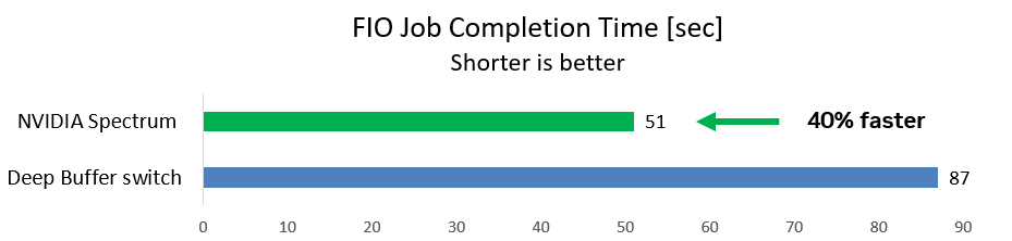
The first case uses a common storage benchmarking FIO tool for WRITE operations from two initiators to one target while background traffic is running. This is a typical storage scenario. 

The team measured the time required for the FIO job to complete (shorter is better). With the deep-buffer switch, the FIO job took 87 seconds. With the NVIDIA Spectrum switch, the job ran 40% faster and completed after just 51 seconds.

Deep-buffer switches greatly increase latency, which slows down your storage and reduces your application performance. But how high can the latency go?

For the second case, the team took the deep-buffer switch and tested how latency is impacted under different congestion use cases. The maximum buffer occupancy is only around 10% of the whole buffer size.

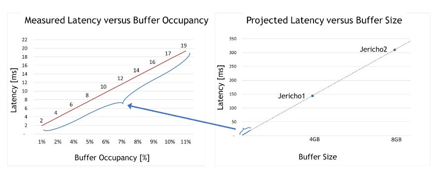
Two meaningful insights can be derived from the graph on the left of Figure 2. First, deep-buffer switch latency is 50,000x higher than Spectrum switches (2–19 milliseconds compared to only 300 nanoseconds for Spectrum). 

Second, linear dependency is apparent between buffer occupancy and latency. In other words, testing proved that the larger the occupied buffer, the greater the latency.

With that understanding, the graph on the right of Figure 2 projects the maximum latency per deep-buffer ASIC (such as Jericho 1, Jericho 2, or Ramon). These very high latency numbers are incompatible with data center applications in general and fast storage solutions in particular.

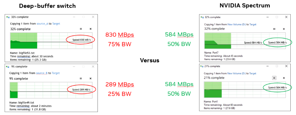
For the third case, the team used two Windows machines and simultaneously copied a file from each to the same target storage.

With the deep-buffer switch, one Windows machine had three times the bandwidth of the other (830 MBps compared to 290 MBps). With Spectrum switch, each machine had 584 MBps (50% as expected).

Real-world testing showed that deep-buffer switches do not have a positive impact on data center applications, such as absorbing packets and preventing drops.

Deep-buffer switches may be needed for long haul or WAN connections; however, they are suboptimal for data center applications and will have negative effects, particularly when the workload is scaled beyond just two nodes, as in this use case. 

These three use cases demonstrate proof points for why deep-buffer switches adversely impact AI/ML and storage workloads, while Spectrum switches provide maximized performance.

Summary

NVIDIA Spectrum Ethernet switches are built for AI/ML and storage workloads, and perform better than switches with split buffers or deep buffers. They handle congestion better, prevent packet loss, and outperform with jumbo frames (preferred for storage). NVIDIA Spectrum Ethernet switches provide overall good application performance with consistently low network latency.

Learn more about NVIDIA Spectrum Ethernet switches. Dive deeper into networking storage in the NVIDIA Developer Forums.