Heterogeneous computing architectures—those that incorporate a variety of processor types working in tandem—have proven extremely valuable in the continued…
Heterogeneous computing architectures—those that incorporate a variety of processor types working in tandem—have proven extremely valuable in the continued scalability of computational workloads in AI, machine learning (ML), quantum physics, and general data science.
Critical to this development has been the ability to abstract away the heterogeneous architecture and promote a framework that makes designing and implementing such applications more efficient. The most well-known programming model that accomplishes this is CUDA Toolkit, which enables offloading work to thousands of GPU cores in parallel following a single-instruction, multiple-data model.
Recently, a new form of node-level coprocessor technology has been attracting the attention of the computational science community: the quantum computer, which relies on the non-intuitive laws of quantum physics to process information using principles such as superposition, entanglement, and interference. This unique accelerator technology may prove useful in very specific applications and is poised to work in tandem with CPUs and GPUs, ushering in an era of computational advances previously deemed unfeasible.
The question then becomes: If you enhance an existing classically heterogeneous compute architecture with quantum coprocessors, how would you program it in a manner fit for computational scalability?
NVIDIA is answering this question with CUDA Quantum, an open-source programming model extending both C++ and Python with quantum kernels intended for compilation and execution on quantum hardware.
This post introduces CUDA Quantum, highlights its unique features, and demonstrates how researchers can leverage it to gather momentum in day-to-day quantum algorithmic research and development.
CUDA Quantum: Hello quantum world
To begin with a look at the CUDA Quantum programming model, create a two-qubit GHZ state with the Pythonic interface. This will accustom you to its syntax.
import cudaq

# Create the CUDA Quantum Kernel
kernel = cudaq.make_kernel()

# Allocate 2 qubits
qubits = kernel.qalloc(2)

# Prepare the bell state
kernel.h(qubits[0])
kernel.cx(qubits[0], qubits[1])

# Sample the final state generated by the kernel
result = cudaq.sample(kernel, shots_count = 1000)

print(result)

{11:487, 00:513}
The language specification borrows concepts that CUDA has proven successful; specifically, the separation of host and device code at the function boundary level. The code snippet below demonstrates this functionality on a GHZ state preparation example in C++.
#include

int main() {
      // Define the CUDA Quantum kernel as a C++ lambda
	auto ghz =[](int numQubits) __qpu__ {
           // Allocate a vector of qubits
		cudaq::qvector q(numQubits);

           // Prepare the GHZ state, leverage standard
           // control flow, specify the x operation
           // is controlled.
		h(q[0]);
		for (int i = 0; i (q[i], q[i + 1]);
	};

     // Sample the final state generated by the kernel
auto results = cudaq::sample(ghz, 15);
results.dump();

return 0;
}
CUDA Quantum enables the definition of quantum code as stand-alone kernel expressions. These expressions can be any callable in C++ (a lambda is shown here, and implicitly typed callable) but must be annotated with the __qpu__ attribute enabling the nvq++ compiler to compile them separately. Kernel expressions can take classical input by value (here the number of qubits) and leverage standard C++ control flow, for example for loops and if statements.
The utility of GPUs
The experimental efforts to scale up QPUs and move them out of research labs and host them on the cloud for general access have been phenomenal. However, current QPUs are noisy and small-scale, hindering advancement of algorithmic research. To aid this, circuit simulation techniques are answering the pressing requirements to advance research frontiers.
Desktop CPUs can simulate small-scale qubit statistics; however, memory requirements of the state vector grow exponentially with the number of qubits. A typical desktop computer possesses eight GB of RAM, enabling one to sluggishly simulate approximately 15 qubits. The latest NVIDIA DGX H100 enables you to surpass the 35-qubit mark with unparalleled speed.
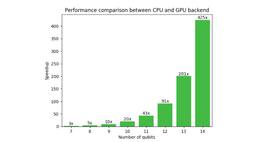
Figure 1 shows a comparison of CUDA Quantum on CPU and GPU backend for a typical variational algorithmic workflow. The need for GPUs is evident here, as the speedup at 14 qubits is 425x and increases with qubit count. Extrapolating to 30 qubits, the CPU-to-GPU runtime is 13 years, compared to 2 days. This unlocks researchers’ abilities to go beyond small-scale proof of concept results to implementing algorithms closer to real-world applications.
Along with CUDA Quantum, NVIDA has developed cuQuantum, a library enabling lightning-fast simulation of a quantum computer using both state vector and tensor network methods through hand-optimized CUDA kernels. Memory allocation and processing happens entirely on GPUs resulting in dramatic increases in performance and scale. CUDA Quantum in combination with cuQuantum forms a powerful platform for hybrid algorithm research.
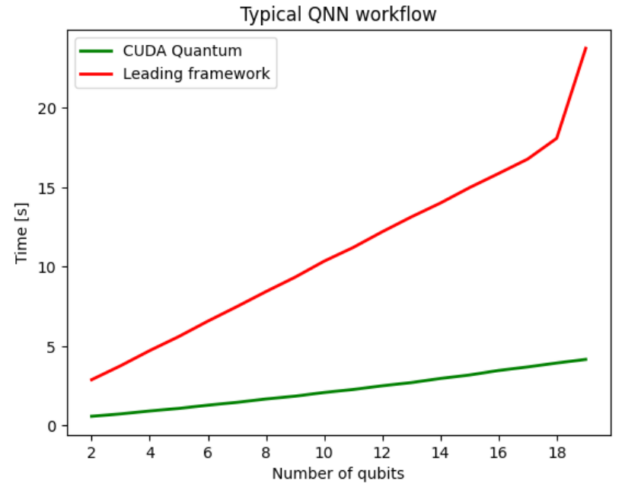
Figure 2 compares CUDA Quantum with a leading quantum computing SDK, both leveraging the NVIDIA cuQuantum backend to optimally offload circuit simulation onto NVIDIA GPUs. In this case, the benefits of using CUDA Quantum are isolated and yield a 5x performance improvement on average compared to a leading framework.
Enabling multi-QPU workflows of the future
CUDA Quantum is not limited to consideration of current cloud-based quantum execution models, but is fully anticipating tightly coupled, system-level quantum acceleration. Moreover, CUDA Quantum enables application developers to envision workflows for multi-QPU architectures with multi-GPU backends.
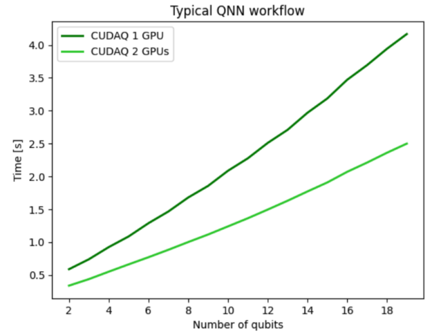
For the preceding quantum neural network (QNN) example, you can use the multi-GPU functionality to run a forward pass of the dataset enabling us to perform multi-QPU workflows of the future. Figure 3 shows results for distributing the QNN workflow across two GPUs and demonstrates strong scaling performance indicating effective usage of all GPU compute resources. Using two GPUs makes the overall workflow twice as fast compared to a single GPU, demonstrating strong scaling.
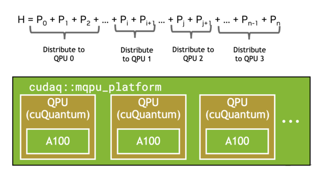
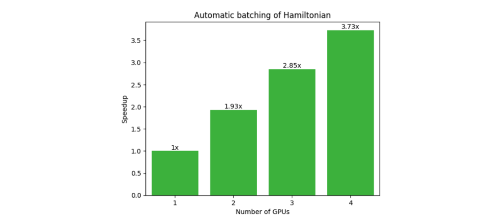
Another common workflow that benefits from multi-QPU parallelization is the Variational Quantum Eigensolver (VQE). This requires the expectation value of a composite Hamiltonian made up of multiple single Pauli tensor product terms. The CUDA Quantum observe call, shown below, automatically batches terms (Figure 4), and offloads to multiple GPUs or QPUs if available, demonstrating strong scaling (Figure 5).
numQubits, numTerms = 30, 1e5
hamiltonian = cudaq.SpinOperator.random(numQubits, numTerms)
cudaq.observe(ansatz, hamiltonian, parameters)
GPU-QPU workflows
This post has so far explored using GPUs for scaling quantum circuit simulation beyond what is possible on CPUs, as well as multi-QPU workflows. The following sections dive into true heterogeneous computing with a hybrid quantum neural network example using PyTorch and CUDA Quantum.
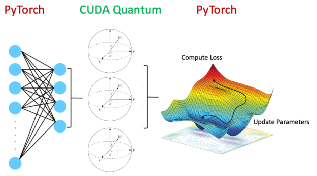
As shown in Figure 6, a hybrid quantum neural network encompasses a quantum circuit as a layer within the overall neural network architecture. An active area of research, this is poised to be advantageous in certain areas, improving generalization errors.
Evidently, it is advantageous to run the classical neural network layers on GPUs and the quantum circuits on QPUs. Accelerating the whole workflow with CUDA Quantum is made possible by setting the following:
quantum_device = cudaq.set_target('ion-trap')
classical_device = torch.cuda.set_device(gpu0)
The utility of this is profound. CUDA Quantum enables offloading relevant kernels suited for QPUs and GPUs in a tightly integrated, seamless fashion. In addition to hybrid applications, workflows involving error correction, real-time optimal control, and error mitigation through Clifford data regression would all benefit from tightly coupled compute architectures.
QPU hardware providers
The foundational information unit embedded within the CUDA Quantum programming paradigm is the qudit, which represents a quantum bit capable of accessing d-states. Qubit is a specific instance where d=2. By using qudits, CUDA Quantum can efficiently target diverse quantum computing architectures, including superconducting circuits, ion traps, neutral atoms, diamond-based, photonic systems, and more.
You can conveniently develop workflows, and the nvq++ compiler automatically compiles and executes the program on the designated architecture. Figure 7 shows the compilation speedups that the novel compiler yields. Compilation involves circuit optimization, decomposing into the native gate sets supported by the hardware and qubit routing. The nvq++ compiler used by CUDA Quantum is on average 2.4x faster compared to its competition.

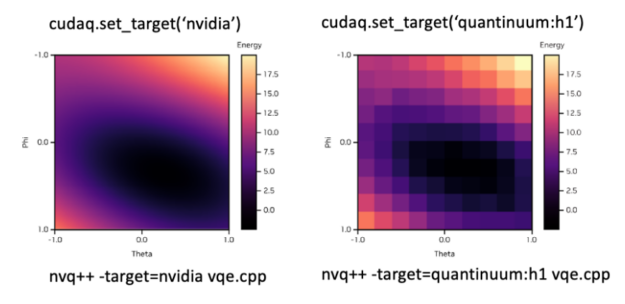
To accommodate the desired backend, you can simply modify the set_target() flag. Figure 8 shows an example of how you can seamlessly switch between the simulated backend and the Quantinuum H1 ion trap system. The top shows the syntax to set the desired backend in Python and the bottom in C++.
Getting started with CUDA Quantum
This post has just briefly touched on some of the features of the CUDA Quantum programming model. Reach out to the CUDA Quantum community on GitHub and get started with some example code snippets. We are excited to see the research CUDA Quantum enables for you.


 Pipeline state objects (PSOs) define how input data is interpreted and rendered by the hardware when submitting work to the GPUs. Proper management of PSOs is…
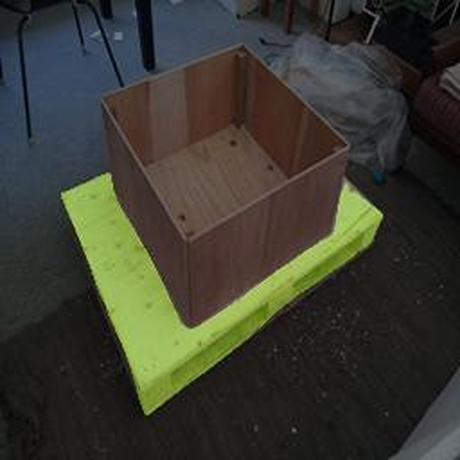
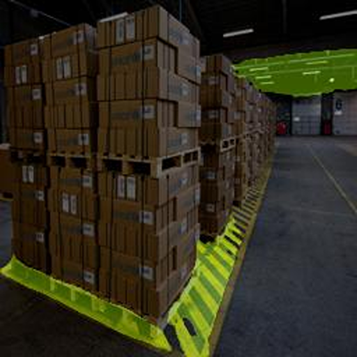
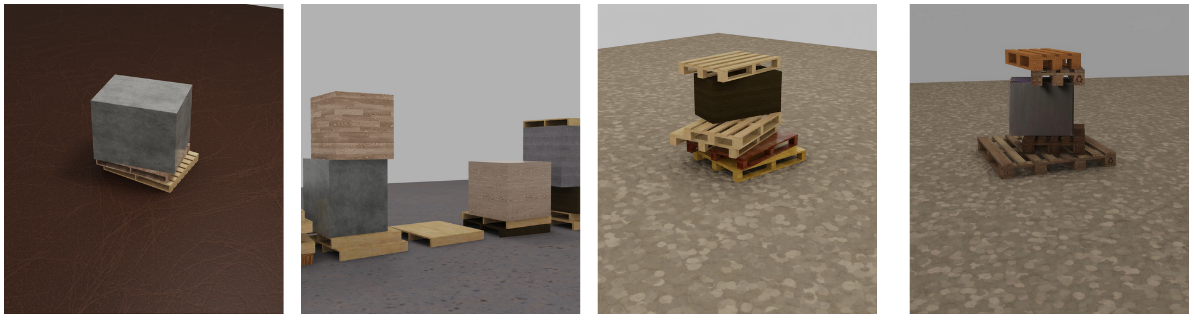
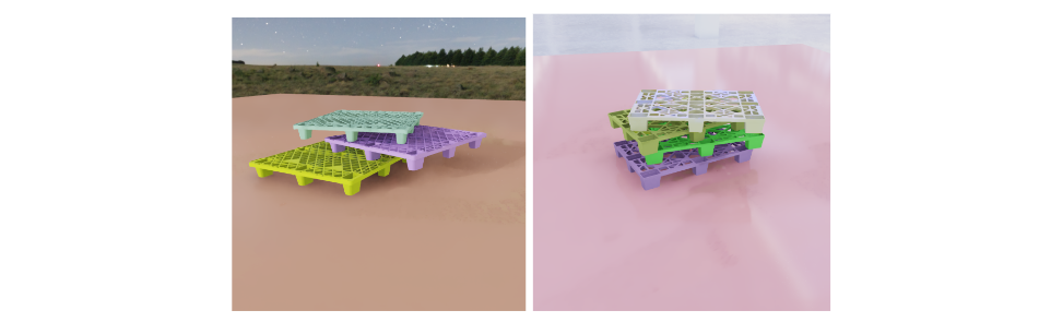
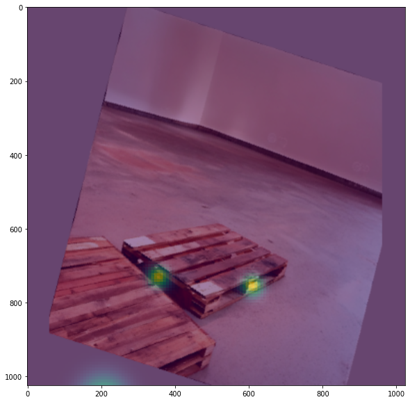
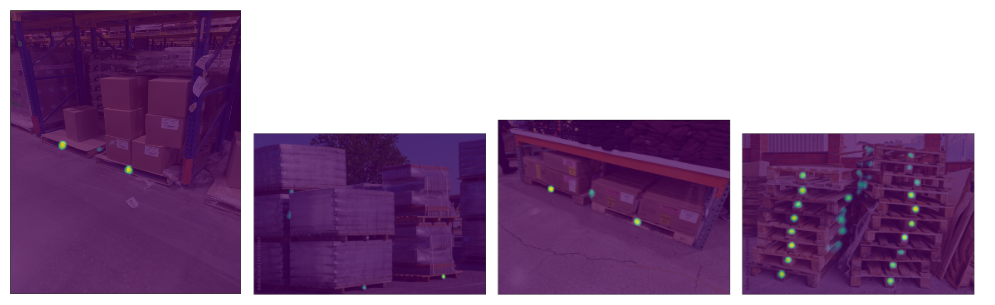
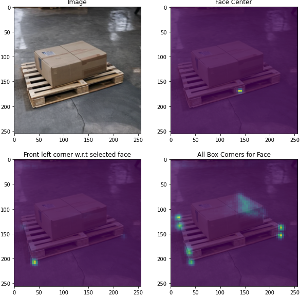
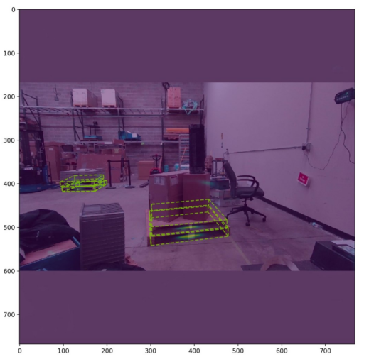
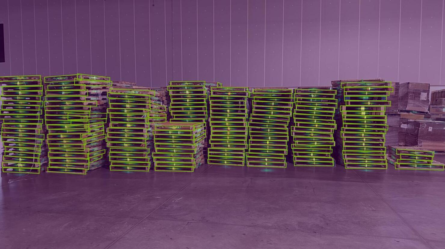
 Imagine you are a robotics or machine learning (ML) engineer tasked with developing a model to detect pallets so that a forklift can manipulate them. You are…
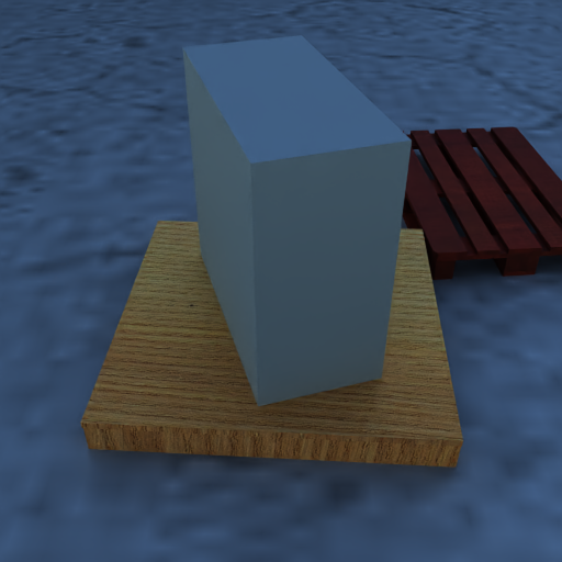

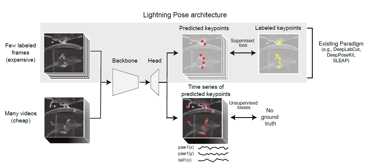
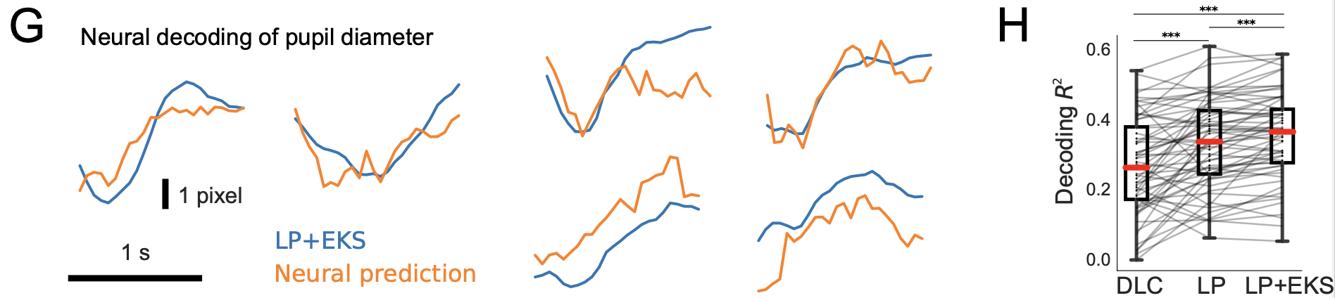
 A primary goal in the field of neuroscience is understanding how the brain controls movement. By improving pose estimation, neurobiologists can more precisely…
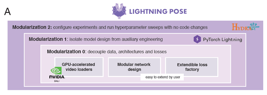
 Gathering business insights can be a pain, especially when you’re dealing with countless data points. It’s no secret that GPUs can be a time-saver for…
 We were stuck. Really stuck. With a hard delivery deadline looming, our team needed to figure out how to process a complex extract-transform-load (ETL) job on…