
A diverse range of artists, fashionistas, musicians and the cinematic arts inspired the creative journey of Pedro Soares, aka Blendeered, and helped him fall in love with using 3D to create art.
China electric vehicle maker XPENG Motors has announced its new G6 coupe SUV — featuring an NVIDIA-powered intelligent advanced driver assistance system — is now available to the China market. The G6 is XPENG’s first model featuring the company’s proprietary Smart Electric Platform Architecture (SEPA) 2.0, which aims to reduce development and manufacturing costs and Read article >
Three leading European generative AI startups joined NVIDIA founder and CEO Jensen Huang this week to talk about the new era of computing. More than 500 developers, researchers, entrepreneurs and executives from across Europe and further afield packed into the Spindler and Klatt, a sleek, riverside gathering spot in Berlin. Huang started the reception by Read article >
The increased frequency and severity of extreme weather and climate events could take a million lives and cost $1.7 trillion annually by 2050, according to the Munich Reinsurance Company. This underscores a critical need for accurate weather forecasting, especially with the rise in severe weather occurrences such as blizzards, hurricanes and heatwaves. AI and accelerated Read article >
Categories
Event: CUDA 12.2 YouTube Premiere
 On July 6, join experts for a deep dive into CUDA 12.2, including support for confidential computing.
On July 6, join experts for a deep dive into CUDA 12.2, including support for confidential computing.
 Deep learning is achieving significant success in various fields and areas, as it has revolutionized the way we analyze, understand, and manipulate data. There…
Deep learning is achieving significant success in various fields and areas, as it has revolutionized the way we analyze, understand, and manipulate data. There are many success stories in computer vision, natural language processing (NLP), medical diagnosis and health care, autonomous vehicles, recommendation systems, and climate and weather modeling.
In an era of ever-growing neural network models, the high demand for computational speed becomes a big challenge for hardware and software. Model pruning and low-precision inference are useful solutions.
Starting with the NVIDIA Ampere architecture and the introduction of the A100 Tensor Core GPU, NVIDIA GPUs have the fine-grained structured sparsity feature, which can be used to accelerate inference. For more information, see the NVIDIA A100 Tensor Core GPU Architecture: Unprecedented Acceleration at Every Scale whitepaper.
In this post, we introduce some training recipes for such sparse models to maintain accuracy, including the basic recipes, the progressive recipes, and the combination with int8 quantization. We also discuss how to do the inference with the structured sparsity in the NVIDIA Ampere architecture.
Tencent’s Machine Learning Platform department (MLPD) used the progressive training techniques to simplify training and achieve better accuracy. With the sparsity feature and some quantization techniques, they achieved 1.3–1.8x acceleration in Tencent’s offline services.
Structured sparsity in the NVIDIA Ampere architecture
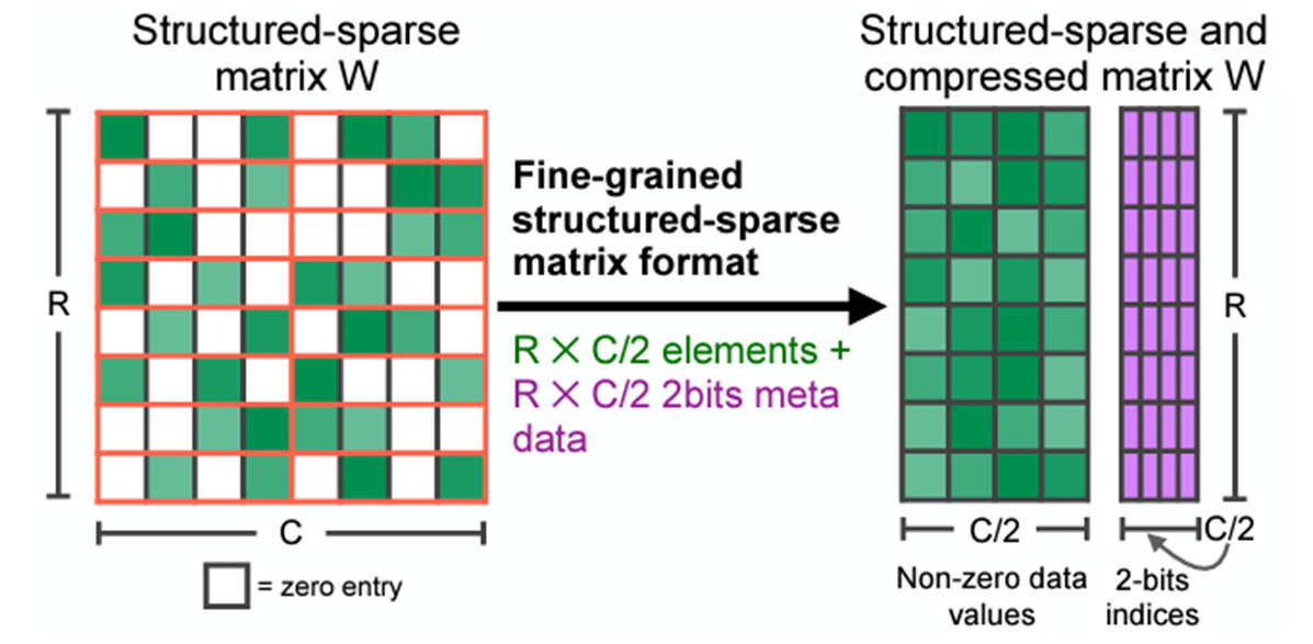
NVIDIA Ampere and NVIDIA Hopper architecture GPUs add the new feature of fine-grained structured sparsity, which can mainly be used to accelerate inference workloads. This feature is supported by sparse Tensor Cores, which require a 2:4 sparsity pattern. Among each group of four contiguous values, at least two must be zero, which is a 50% sparsity rate.
This pattern can have efficient memory access, good speedup, and can easily recover accuracy. After compression, only non-zero values and the associated index metadata are stored (Figure 1). The sparse Tensor Cores process only the non-zero values when doing matrix multiplication and theoretically, the compute throughput would be 2x compared to the equivalent dense matrix multiplication.
Structured sparsity can mainly be applied on fully connected layers and convolution layers where 2:4 sparse weights are provided. If you prune the weights of these layers in advance, then these layers can be accelerated by structured sparsity.
Training recipes
As directly pruning the weights decreases the model accuracy, you should do some training to recover the accuracy when using the structured sparsity. Here, we introduce some basic recipes and new progressive recipes.
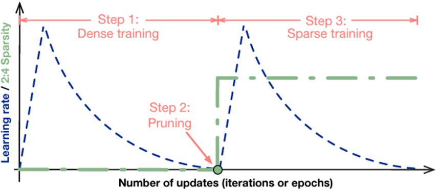
Basic recipes
The basic recipes maintain the model accuracy without any hyperparameter tuning. For more information, see Accelerating Sparse Deep Neural Networks.
The workflow is easy to follow:
- Train a model without sparsity.
- Prune the model in a 2:4 sparse pattern for the FC and convolution layers.
- Retrain the pruned model by following these rules:
- Initialize the weights to the values from Step 2.
- Use the same optimizer and hyperparameter (learning rate, schedule, number of epochs, and so on) as in Step 1.
- Maintain the sparsity pattern computed in Step 2.
There are also some advanced recipes for complicated cases.
For example, apply sparse training in multiple stages. For some object detection models, if the dataset in the downstream task is large enough, you can just repeat the fine-tuning with sparsity. For models like BERT-SQuAD, the dataset is relatively small, and you must apply the sparsity to the pretraining phase for better accuracy.
Also, you can easily combine the sparsity training with int8 QAT by inserting the quant nodes before fine-tuning. All these training and fine-tuning methods are one-shot, as the final model is obtained after one sparse training process.
Progressive training recipes
One-shot sparse fine-tuning can cover most tasks and achieve speedup without accuracy loss. On the other hand, for some difficult tasks that are sensitive to weight changes, one-shot sparsity for all weights causes large information loss. It’s difficult to recover accuracy by only fine-tuning with small datasets, and sparse pretraining is also needed for these tasks.
Sparse pretraining requires more data and is more time-consuming. So, inspired by the pruning method for CNN, the progressive sparsity is introduced to apply sparsity only on fine-tuning phase for such tasks without too much accuracy loss. For more information, see Learning Both Weights and Connections for Efficient Neural Networks.

The key idea of progressive sparsity is to divide the target sparsity ratio into several small steps.
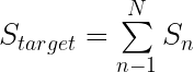
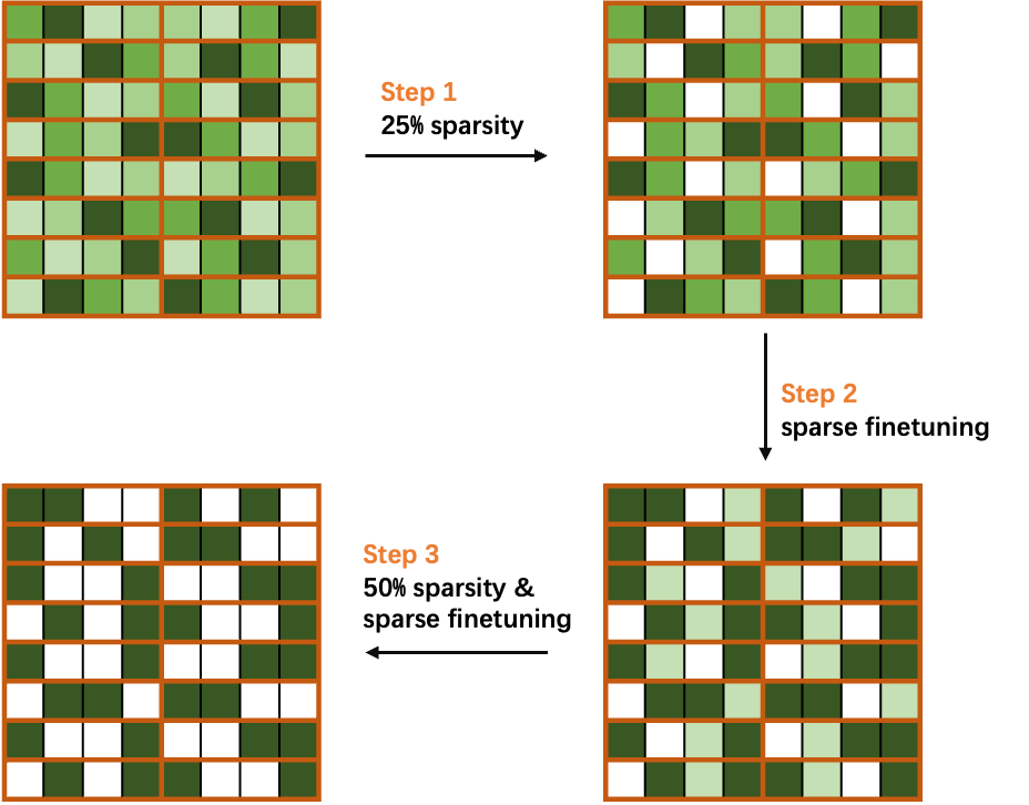
As shown in the equation and Figure 4, for a target sparsity ratio S, you divide it into N steps, which facilitates the rapid recovery of information during the fine-tuning process. Based on our experiments, progressive sparsity can achieve higher accuracy than one-shot sparsity with the same fine-tuning epochs.
Taking 50% sparsity in a 2:4 pattern as a simple case, divide the sparsity ratio into two steps, and progressively sparse and fine-tune the weights in the network.
As shown in Figure 4, you first compute the mask of weights to achieve 25% sparsity, and then perform sparse fine-tuning to recover the accuracy. Finally, you recalculate the mask to 50% sparsity and fine-tuning the network to obtain a sparse model without loss of accuracy.
Sparse-QAT: Combine sparsity with quantization and distillation
To obtain lighter models, you can further combine sparsity with quantization and distillation in a method called sparse-QAT.
Quantization (PTQ and QAT)
The following equation formulates a general quantization procedure. For a float32 value x, use ![Q[x]](https://s0.wp.com/latex.php?latex=Q%5Bx%5D&bg=transparent&fg=000&s=0&c=20201002)
![Q[x] = s times round bigl( clamp left( frac{x}{s},l_{min},l_{max} right) bigr)](https://s0.wp.com/latex.php?latex=Q%5Bx%5D+%3D+s+%5Ctimes+round+%5Cbigl%28+clamp+%5Cleft%28+%5Cfrac%7Bx%7D%7Bs%7D%2Cl_%7Bmin%7D%2Cl_%7Bmax%7D+%5Cright%29+%5Cbigr%29&bg=transparent&fg=000&s=2&c=20201002)
In general, you first quantize the original parameters to a certain range and round them to integers. Then, you use the quantization scale to recover the original value. This motivates your first quantization method, calibration, also known as post-training quantization (PTQ).
In calibration, a critical thing is to set an appropriate quantization scale. If the scale is too large, it is less accurate for numbers within the range. On the contrary, if the scale is too small, it results in too many numbers outside the range of 

Therefore, to balance these two aspects, you first obtain the distribution of tensor values and then set the quantization scale to include 99.99% of the numbers. It has been proved in multiple works that this method is helpful in finding a good quantization scale during calibration.
However, although you have set a reasonable quantization scale for calibration, the accuracy still drops significantly for 8 bits. You then introduce quantization-aware training (QAT) to further improve the accuracy after calibration. The idea of QAT is to train a model with simulation quantization.
In the forward pass, you quantize the weights to int8 and dequantize them to float in the node to simulate quantization. In the backward pass, the gradients are used to update the model weights, which is called straight-through estimation (STE). The key idea is the following equation:
![frac{partial f}{partial x} = frac{partial f }{partial Q[x] }](https://s0.wp.com/latex.php?latex=%5Cfrac%7B%5Cpartial+f%7D%7B%5Cpartial+x%7D+%3D+%5Cfrac%7B%5Cpartial+f+%7D%7B%5Cpartial+Q%5Bx%5D+%7D&bg=transparent&fg=000&s=4&c=20201002)
Gradients of values in the threshold ranges are passed directly in the backward pass, and gradients of values outside the threshold ranges are clipped to 0.
Knowledge distillation
In addition to the previous methods, we introduced knowledge distillation (KD) to further ensure the accuracy of the sparse-QAT model. Take the original model as the teacher and the quantized sparse model as the student.
During the fine-tuning process, we adopted mini-distillation, which is a layer-wise distillation. With MiniLM, you only have to use the self-attention output of the last transformer layer to do the distillation. You can even achieve higher accuracy than the teacher model after Sparse-QAT. For more information, see MiniLM: Deep Self-Attention Distillation for Task-Agnostic Compression of Pre-Trained Transformers.
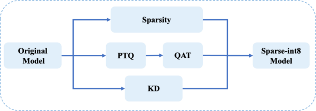
Pipeline of Sparse-QAT
Figure 5 shows the pipeline of Sparse-QAT. You use sparsity, quantization, and KD together to get the final sparse-int8 model. There are three passes:
- Sparsity pass: Apply progressive sparsity to get a sparse tensor.
- Quantization pass: Use PTQ and QAT to get an int8 tensor.
- Knowledge distillation pass: Use MiniLM to guarantee the accuracy of the final sparse-int8 model.
Inference with NVIDIA Ampere architecture sparsity
After the sparse model is trained, you can use TensorRT and cuSPARSELt to accelerate the inference with NVIDIA Ampere architecture structured sparsity.
Inference with NVIDIA TensorRT
NVIDIA TensorRT supports sparse convolution as of version 8.0. GEMMs should be replaced with 1×1 convolutions to use the sparsity inference. Enabling sparsity in TensorRT is easy. Before importing into TensorRT, the weights of the model should have 2:4 sparsity. If trtexec is used to build the engine, set the –sparsity=enable flag. If you are writing codes or scripts to build the engine, set the build config as follows:
For C++: config->setFlag(BuilderFlag::kSPARSE_WEIGHTS)
For Python: config.set_flag(trt.BuilderFlag.SPARSE_WEIGHTS)
Use NVIDIA cuSPARSELt to enhance TensorRT
For some use cases, the input sizes may vary and TensorRT may not provide the best performance. You can use NVIDIA cuSPARSELt to further accelerate these cases.
The solution is to write TensoRT plug-ins with cuSPARSELt. Initialize multiple descriptors and plans of cuSPARSELt sparse GEMM for different input sizes and choose an appropriate plan for each input.
Assuming that you implement the SpmmPluginDynamic plug-in, it inherits from nvinfer1::IPluginV2DynamicExt and you use a private struct to store the plans.
 struct cusparseLtContext {
    cusparseLtHandle_t handle;
    std::vector plans;
    std::vector matAs, matBs, matCs;
    std::vector matmuls;
    std::vector alg_sels;
}
A TensorRT plug-in should implement the configurePlugin method, which sets up the plug-in according to the input and output types and sizes. You initialize the cuSPARSELt-related structures in this method.
There is a constraint that the input size of cuSPARSELt should be a multiple of 4, 8, or 16 depending on the data type. For this post, we set it to a multiple of 16. For more information about the constraints, see cusparseLtDenseDescriptorInit.
for (int i = 0; i
In the enqueue function, you can select the proper plan to do the matmul operation:
int m = inputDesc->dims.d[0];
int idx = (m + 15) / 16 - 1;
float alpha = 1.0f;
float beta = 0.0f;
auto input = static_cast(inputs[0]);
auto output = static_cast(outputs[0]);
cusparseStatus_t status = cusparseLtMatmul(
    &handle, &plans[idx], &alpha, input,
    weight_compressed, &beta, output, output, workSpace, &stream, 1);
Some applications in search engines
In this section, we show four applications that take advantage of sparsity in search engines:
- Search relevance prediction aims to evaluate the relevance between the input text and the videos in the database.
- Query performance prediction is used for the document recall delivery strategy.
- A recall task for recalling the most relevant texts.
- The text-to-image task automatically generates corresponding pictures according to the input prompt.
Search relevance cases
The results of these cases are evaluated with positive negative rate (PNR) or accuracy (Acc).
In relevance case 1, we ran Sparse-QAT and obtained a sparse-int8 model with higher PNR than the online int8 model in two important evaluation indices.
| Model | Evaluation Index A | Evaluation Index B |
| float32 | 4.0138 | 3.1384 |
| int8 (online) | 3.9454 | 2.9120 |
| Sparse-int8 | 4.0406 | 2.9591 |
In relevance case 2, the sparse-int8 model can achieve comparable Acc scores to the float32 model with a 1.4x inference speedup compared to the dense-int8 model.
| Evaluation Index | |
| Bert_12L (float32) | 0.8015 |
| Bert_12L (sparse-int8) | 0.8010 |
Query performance prediction cases
In this section, we show four cases of query performance prediction (QPP) that are evaluated with normalized discounted cumulative gain (NDCG). As shown in Table 3, these sparse-fp16 models can achieve even higher accuracy than the original float32 models, with a four-fold speedup in inference and negligible impact on the NDCG.
| Case A | Case B | Case C | Case D | |
| NDCG (float32 model) |
39723 | 39858 | 39878 | 32471 |
| NDCG (sparse-float16) |
39744 | 39927 | 39909 | 32494 |
| Relative inference time (float32) | 1 | 1 | 1 | 1 |
| Relative inference time (sparse-float16) | 0.25 | 0.25 | 0.25 | 0.25 |
| Inference speedup | 4x | 4x | 4x | 4x |
Query-doc case
Table 4 shows the result of a query-doc case in the search engine. With the proposed sparse-QAT pipeline, the sparse-int8 models can achieve 1.4x inference speedup with negligible accuracy loss compared with the dense-int8 model.
| Acc | f1_345 | recall_345 | |
| FP32 model | 0.7839 | 0.8627 | 0.8312 |
| Sparse-int8 model | 0.7814 | 0.8622 | 0.8416 |
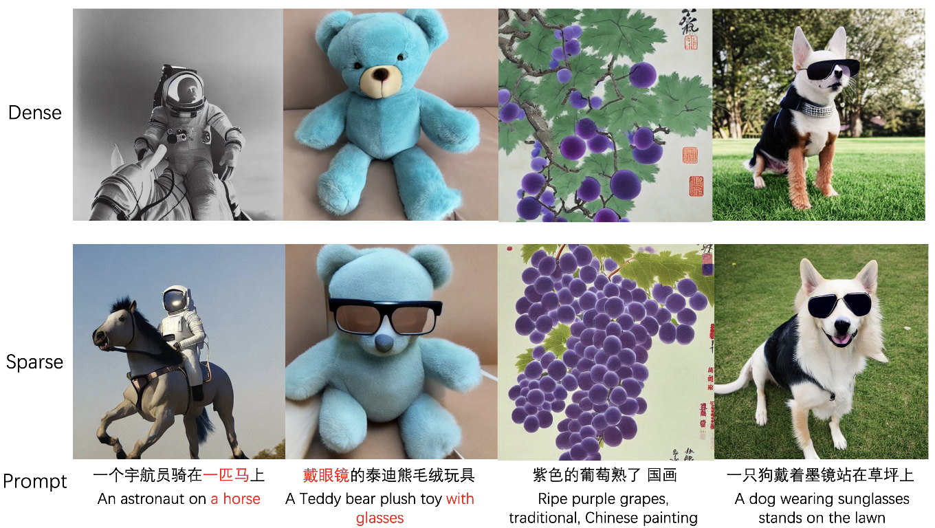
Text-to-image cases
Figure 6 shows the results of text-to-image models. The top four images are the output of the dense float32 model, and the bottom four images are the output of the sparse float16 model.
From the results, you can see that, given the same prompt, the sparse model can produce comparable results with the ones from the dense model. Some of the results are more reasonable as the model pruning and extra progressive sparse fine-tuning make the model learn more from the data.
Summary
The structured sparsity feature in the NVIDIA Ampere architecture can accelerate many deep learning workloads, and it is easy to use with TensorRT and cuSPARSELt.
For more information, see the Structured Sparsity in the NVIDIA Ampere Architecture and its Applications in Tencent WeChat Search GTC session. Download the latest TensorRT and cuSPARSELt versions.
AI and accelerated computing will help climate researchers achieve the miracles they need to achieve breakthroughs in climate research, NVIDIA founder and CEO Jensen Huang said during a keynote Monday at the Berlin Summit for the Earth Virtualization Engines initiative. “Richard Feynman once said that “what I can’t create, I don’t understand” and that’s the Read article >
Deep learning has recently driven tremendous progress in a wide array of applications, ranging from realistic image generation and impressive retrieval systems to language models that can hold human-like conversations. While this progress is very exciting, the widespread use of deep neural network models requires caution: as guided by Google’s AI Principles, we seek to develop AI technologies responsibly by understanding and mitigating potential risks, such as the propagation and amplification of unfair biases and protecting user privacy.
Fully erasing the influence of the data requested to be deleted is challenging since, aside from simply deleting it from databases where it’s stored, it also requires erasing the influence of that data on other artifacts such as trained machine learning models. Moreover, recent research [1, 2] has shown that in some cases it may be possible to infer with high accuracy whether an example was used to train a machine learning model using membership inference attacks (MIAs). This can raise privacy concerns, as it implies that even if an individual’s data is deleted from a database, it may still be possible to infer whether that individual’s data was used to train a model.
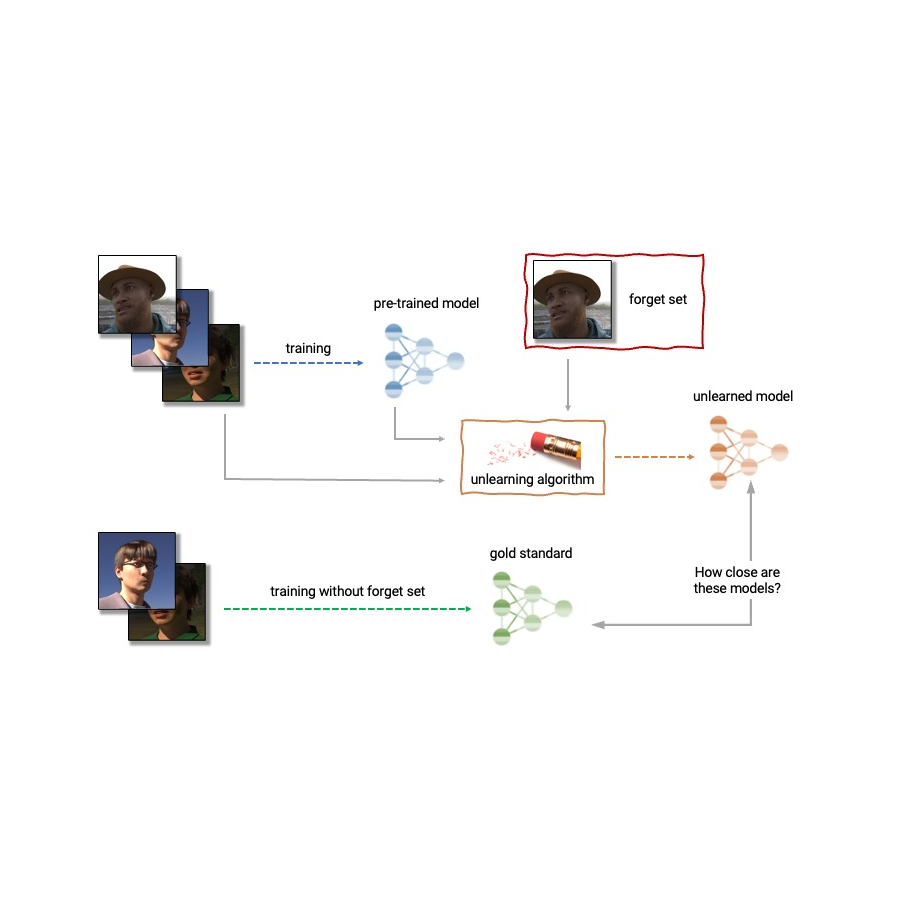
Given the above, machine unlearning is an emergent subfield of machine learning that aims to remove the influence of a specific subset of training examples — the “forget set” — from a trained model. Furthermore, an ideal unlearning algorithm would remove the influence of certain examples while maintaining other beneficial properties, such as the accuracy on the rest of the train set and generalization to held-out examples. A straightforward way to produce this unlearned model is to retrain the model on an adjusted training set that excludes the samples from the forget set. However, this is not always a viable option, as retraining deep models can be computationally expensive. An ideal unlearning algorithm would instead use the already-trained model as a starting point and efficiently make adjustments to remove the influence of the requested data.
Today we’re thrilled to announce that we’ve teamed up with a broad group of academic and industrial researchers to organize the first Machine Unlearning Challenge. The competition considers a realistic scenario in which after training, a certain subset of the training images must be forgotten to protect the privacy or rights of the individuals concerned. The competition will be hosted on Kaggle, and submissions will be automatically scored in terms of both forgetting quality and model utility. We hope that this competition will help advance the state of the art in machine unlearning and encourage the development of efficient, effective and ethical unlearning algorithms.
Machine unlearning applications
Machine unlearning has applications beyond protecting user privacy. For instance, one can use unlearning to erase inaccurate or outdated information from trained models (e.g., due to errors in labeling or changes in the environment) or remove harmful, manipulated, or outlier data.
The field of machine unlearning is related to other areas of machine learning such as differential privacy, life-long learning, and fairness. Differential privacy aims to guarantee that no particular training example has too large an influence on the trained model; a stronger goal compared to that of unlearning, which only requires erasing the influence of the designated forget set. Life-long learning research aims to design models that can learn continuously while maintaining previously-acquired skills. As work on unlearning progresses, it may also open additional ways to boost fairness in models, by correcting unfair biases or disparate treatment of members belonging to different groups (e.g., demographics, age groups, etc.).
 |
| Anatomy of unlearning. An unlearning algorithm takes as input a pre-trained model and one or more samples from the train set to unlearn (the “forget set”). From the model, forget set, and retain set, the unlearning algorithm produces an updated model. An ideal unlearning algorithm produces a model that is indistinguishable from the model trained without the forget set. |
Challenges of machine unlearning
The problem of unlearning is complex and multifaceted as it involves several conflicting objectives: forgetting the requested data, maintaining the model’s utility (e.g., accuracy on retained and held-out data), and efficiency. Because of this, existing unlearning algorithms make different trade-offs. For example, full retraining achieves successful forgetting without damaging model utility, but with poor efficiency, while adding noise to the weights achieves forgetting at the expense of utility.
Furthermore, the evaluation of forgetting algorithms in the literature has so far been highly inconsistent. While some works report the classification accuracy on the samples to unlearn, others report distance to the fully retrained model, and yet others use the error rate of membership inference attacks as a metric for forgetting quality [4, 5, 6].
We believe that the inconsistency of evaluation metrics and the lack of a standardized protocol is a serious impediment to progress in the field — we are unable to make direct comparisons between different unlearning methods in the literature. This leaves us with a myopic view of the relative merits and drawbacks of different approaches, as well as open challenges and opportunities for developing improved algorithms. To address the issue of inconsistent evaluation and to advance the state of the art in the field of machine unlearning, we’ve teamed up with a broad group of academic and industrial researchers to organize the first unlearning challenge.
Announcing the first Machine Unlearning Challenge
We are pleased to announce the first Machine Unlearning Challenge, which will be held as part of the NeurIPS 2023 Competition Track. The goal of the competition is twofold. First, by unifying and standardizing the evaluation metrics for unlearning, we hope to identify the strengths and weaknesses of different algorithms through apples-to-apples comparisons. Second, by opening this competition to everyone, we hope to foster novel solutions and shed light on open challenges and opportunities.
The competition will be hosted on Kaggle and run between mid-July 2023 and mid-September 2023. As part of the competition, today we’re announcing the availability of the starting kit. This starting kit provides a foundation for participants to build and test their unlearning models on a toy dataset.
The competition considers a realistic scenario in which an age predictor has been trained on face images, and, after training, a certain subset of the training images must be forgotten to protect the privacy or rights of the individuals concerned. For this, we will make available as part of the starting kit a dataset of synthetic faces (samples shown below) and we’ll also use several real-face datasets for evaluation of submissions. The participants are asked to submit code that takes as input the trained predictor, the forget and retain sets, and outputs the weights of a predictor that has unlearned the designated forget set. We will evaluate submissions based on both the strength of the forgetting algorithm and model utility. We will also enforce a hard cut-off that rejects unlearning algorithms that run slower than a fraction of the time it takes to retrain. A valuable outcome of this competition will be to characterize the trade-offs of different unlearning algorithms.
 |
| Excerpt images from the Face Synthetics dataset together with age annotations. The competition considers the scenario in which an age predictor has been trained on face images like the above, and, after training, a certain subset of the training images must be forgotten. |
For evaluating forgetting, we will use tools inspired by MIAs, such as LiRA. MIAs were first developed in the privacy and security literature and their goal is to infer which examples were part of the training set. Intuitively, if unlearning is successful, the unlearned model contains no traces of the forgotten examples, causing MIAs to fail: the attacker would be unable to infer that the forget set was, in fact, part of the original training set. In addition, we will also use statistical tests to quantify how different the distribution of unlearned models (produced by a particular submitted unlearning algorithm) is compared to the distribution of models retrained from scratch. For an ideal unlearning algorithm, these two will be indistinguishable.
Conclusion
Machine unlearning is a powerful tool that has the potential to address several open problems in machine learning. As research in this area continues, we hope to see new methods that are more efficient, effective, and responsible. We are thrilled to have the opportunity via this competition to spark interest in this field, and we are looking forward to sharing our insights and findings with the community.
Acknowledgements
The authors of this post are now part of Google DeepMind. We are writing this blog post on behalf of the organization team of the Unlearning Competition: Eleni Triantafillou*, Fabian Pedregosa* (*equal contribution), Meghdad Kurmanji, Kairan Zhao, Gintare Karolina Dziugaite, Peter Triantafillou, Ioannis Mitliagkas, Vincent Dumoulin, Lisheng Sun Hosoya, Peter Kairouz, Julio C. S. Jacques Junior, Jun Wan, Sergio Escalera and Isabelle Guyon.
In recent years, diffusion models have shown great success in text-to-image generation, achieving high image quality, improved inference performance, and expanding our creative inspiration. Nevertheless, it is still challenging to efficiently control the generation, especially with conditions that are difficult to describe with text.
Today, we announce MediaPipe diffusion plugins, which enable controllable text-to-image generation to be run on-device. Expanding upon our prior work on GPU inference for on-device large generative models, we introduce new low-cost solutions for controllable text-to-image generation that can be plugged into existing diffusion models and their Low-Rank Adaptation (LoRA) variants.
 |
| Text-to-image generation with control plugins running on-device. |
Background
With diffusion models, image generation is modeled as an iterative denoising process. Starting from a noise image, at each step, the diffusion model gradually denoises the image to reveal an image of the target concept. Research shows that leveraging language understanding via text prompts can greatly improve image generation. For text-to-image generation, the text embedding is connected to the model via cross-attention layers. Yet, some information is difficult to describe by text prompts, e.g., the position and pose of an object. To address this problem, researchers add additional models into the diffusion to inject control information from a condition image.
Common approaches for controlled text-to-image generation include Plug-and-Play, ControlNet, and T2I Adapter. Plug-and-Play applies a widely used denoising diffusion implicit model (DDIM) inversion approach that reverses the generation process starting from an input image to derive an initial noise input, and then employs a copy of the diffusion model (860M parameters for Stable Diffusion 1.5) to encode the condition from an input image. Plug-and-Play extracts spatial features with self-attention from the copied diffusion, and injects them into the text-to-image diffusion. ControlNet creates a trainable copy of the encoder of a diffusion model, which connects via a convolution layer with zero-initialized parameters to encode conditioning information that is conveyed to the decoder layers. However, as a result, the size is large, half that of the diffusion model (430M parameters for Stable Diffusion 1.5). T2I Adapter is a smaller network (77M parameters) and achieves similar effects in controllable generation. T2I Adapter only takes the condition image as input, and its output is shared across all diffusion iterations. Yet, the adapter model is not designed for portable devices.
The MediaPipe diffusion plugins
To make conditioned generation efficient, customizable, and scalable, we design the MediaPipe diffusion plugin as a separate network that is:
- Plugable: It can be easily connected to a pre-trained base model.
- Trained from scratch: It does not use pre-trained weights from the base model.
- Portable: It runs outside the base model on mobile devices, with negligible cost compared to the base model inference.
| Method | Parameter Size | Plugable | From Scratch | Portable | ||||
| Plug-and-Play | 860M* | ✔️ | ❌ | ❌ | ||||
| ControlNet | 430M* | ✔️ | ❌ | ❌ | ||||
| T2I Adapter | 77M | ✔️ | ✔️ | ❌ | ||||
| MediaPipe Plugin | 6M | ✔️ | ✔️ | ✔️ |
| Comparison of Plug-and-Play, ControlNet, T2I Adapter, and the MediaPipe diffusion plugin. * The number varies depending on the particulars of the diffusion model. |
The MediaPipe diffusion plugin is a portable on-device model for text-to-image generation. It extracts multiscale features from a conditioning image, which are added to the encoder of a diffusion model at corresponding levels. When connecting to a text-to-image diffusion model, the plugin model can provide an extra conditioning signal to the image generation. We design the plugin network to be a lightweight model with only 6M parameters. It uses depth-wise convolutions and inverted bottlenecks from MobileNetv2 for fast inference on mobile devices.
 |
| Overview of the MediaPipe diffusion model plugin. The plugin is a separate network, whose output can be plugged into a pre-trained text-to-image generation model. Features extracted by the plugin are applied to the associated downsampling layer of the diffusion model (blue). |
Unlike ControlNet, we inject the same control features in all diffusion iterations. That is, we only run the plugin once for one image generation, which saves computation. We illustrate some intermediate results of a diffusion process below. The control is effective at every diffusion step and enables controlled generation even at early steps. More iterations improve the alignment of the image with the text prompt and generate more detail.
 |
| Illustration of the generation process using the MediaPipe diffusion plugin. |
Examples
In this work, we developed plugins for a diffusion-based text-to-image generation model with MediaPipe Face Landmark, MediaPipe Holistic Landmark, depth maps, and Canny edge. For each task, we select about 100K images from a web-scale image-text dataset, and compute control signals using corresponding MediaPipe solutions. We use refined captions from PaLI for training the plugins.
Face Landmark
The MediaPipe Face Landmarker task computes 478 landmarks (with attention) of a human face. We use the drawing utils in MediaPipe to render a face, including face contour, mouth, eyes, eyebrows, and irises, with different colors. The following table shows randomly generated samples by conditioning on face mesh and prompts. As a comparison, both ControlNet and Plugin can control text-to-image generation with given conditions.
 |
| Face-landmark plugin for text-to-image generation, compared with ControlNet. |
Holistic Landmark
MediaPipe Holistic Landmarker task includes landmarks of body pose, hands, and face mesh. Below, we generate various stylized images by conditioning on the holistic features.
 |
| Holistic-landmark plugin for text-to-image generation. |
Depth
 |
| Depth-plugin for text-to-image generation. |
Canny Edge
 |
| Canny-edge plugin for text-to-image generation. |
Evaluation
We conduct a quantitative study of the face landmark plugin to demonstrate the model’s performance. The evaluation dataset contains 5K human images. We compare the generation quality as measured by the widely used metrics, Fréchet Inception Distance (FID) and CLIP scores. The base model is a pre-trained text-to-image diffusion model. We use Stable Diffusion v1.5 here.
As shown in the following table, both ControlNet and the MediaPipe diffusion plugin produce much better sample quality than the base model, in terms of FID and CLIP scores. Unlike ControlNet, which needs to run at every diffusion step, the MediaPipe plugin only runs once for each image generated. We measured the performance of the three models on a server machine (with Nvidia V100 GPU) and a mobile phone (Galaxy S23). On the server, we run all three models with 50 diffusion steps, and on mobile, we run 20 diffusion steps using the MediaPipe image generation app. Compared with ControlNet, the MediaPipe plugin shows a clear advantage in inference efficiency while preserving the sample quality.
| Model | FID↓ | CLIP↑ | Inference Time (s) | |||||
| Nvidia V100 | Galaxy S23 | |||||||
| Base | 10.32 | 0.26 | 5.0 | 11.5 | ||||
| Base + ControlNet | 6.51 | 0.31 | 7.4 (+48%) | 18.2 (+58.3%) | ||||
| Base + MediaPipe Plugin | 6.50 | 0.30 | 5.0 (+0.2%) | 11.8 (+2.6%) | ||||
| Quantitative comparison on FID, CLIP, and inference time. |
We test the performance of the plugin on a wide range of mobile devices from mid-tier to high-end. We list the results on some representative devices in the following table, covering both Android and iOS.
| Device | Android | iOS | ||||||||||
| Pixel 4 | Pixel 6 | Pixel 7 | Galaxy S23 | iPhone 12 Pro | iPhone 13 Pro | |||||||
| Time (ms) | 128 | 68 | 50 | 48 | 73 | 63 | ||||||
| Inference time (ms) of the plugin on different mobile devices. |
Conclusion
In this work, we present MediaPipe, a portable plugin for conditioned text-to-image generation. It injects features extracted from a condition image to a diffusion model, and consequently controls the image generation. Portable plugins can be connected to pre-trained diffusion models running on servers or devices. By running text-to-image generation and plugins fully on-device, we enable more flexible applications of generative AI.
Acknowledgments
We’d like to thank all team members who contributed to this work: Raman Sarokin and Juhyun Lee for the GPU inference solution; Khanh LeViet, Chuo-Ling Chang, Andrei Kulik, and Matthias Grundmann for leadership. Special thanks to Jiuqiang Tang, Joe Zou and Lu wang, who made this technology and all the demos running on-device.