hey dear, Can you please help me? I saw that you made dots and boxes game in your school project. Actually I have also to make this game and I have the same issue as you. Could you please show me how you did it? Thank you in advance.
Users can now produce 3D virtual worlds at human scale with the new Omniverse XR App available in beta from the NVIDIA Omniverse launcher.
Users can now produce 3D virtual worlds at human scale with the new Omniverse XR App available in beta from the NVIDIA Omniverse launcher.
At Computex this week, NVIDIA announced new releases and expansions to the collaborative graphic platform’s growing ecosystem, including the beta release of Omniverse XR. With this Omniverse app, creators and developers can drop into 3D scenes in VR and AR with full RTX ray tracing. Users can also review, manipulate, and annotate high-poly production assets without preprocessing.
Effortless, ray-traced VR
With the Omniverse XR App users can load Universal Scene Description (USD) production assets directly into the editor. You can jump directly into VR or AR and view or interact with them in ray-traced VR without preprocessing.
Unlike today’s interactive VR engines, Omniverse XR loads USD scenes directly for editing. This removes the need for pregenerated levels of detail since ray tracing is less sensitive to geometry complexity.
The scene below was modeled with 70 million polygons; with instancing, the total scene contains 18 billion polygons.
Figure 1. Production-quality USD-based assets load directly into a scene in Omniverse XR.
Realism out of the box
Fully raytraced VR accounts for a sizable contribution to realism. The human eye notices when contact shadows don’t reflect a scene’s geometry or when reflections don’t move with body motion.
With Omniverse XR, engineers, designers, and researchers are able to see soft shadows, translucency, and real reflections out of the box, making the experience feel truly immersive and realistic.
Figure 2. View a complete 3D scene in VR with the Omniverse XR App.
Navigate and manipulate in VR
Omniverse XR users can teleport and manipulate scene objects in VR. Currently, Oculus and HTC Vive controllers are supported. Since the Omniverse Kit uses real-time ray tracing, ray casting can be done with ease, leading to higher precision in close-range interactions.
Figure 3. Achieve precise object manipulation in Omniverse XR.
Continuous foveated rendering
Omniverse XR uses foveated rendering. This technique samples a region of an HMD screen at a higher shading rate and shrinks the number of pixels rendered to 30% of the image plane. These are pixels that a user won’t see in full resolution.
The foveation technique that comes with Omniverse XR is built specifically for real-time ray tracing. This removes the boundaries between resolution regions, avoiding the need to reshape an image plane when the fovea is off center.
Figure 4. Example of foveated rendering off (left) and on (right).
One-step AR streaming
With Omniverse XR, you can also experience tablet AR streaming, with the NVIDIA CloudXR streaming platform. This mode opens a virtual camera on the tablet, linked to the Omniverse XR session.
To use Tablet AR mode, content creators and developers can download the Omniverse Streaming Client for I/Os. It is available from the Apple Store for iPad I/Os 14.5 and later, or with an APK and code examples available for Android Tablets.
Figure 5. Experience tablet AR streaming.
Explore Omniverse XR
The Omniverse XR App is now available in beta from the Omniverse Launcher. To learn more, check out the tutorial video or attend the Q&A livestream on May 25 at 11 a.m. PDT / 8 p.m. CET.
Additional resources
Learn more by diving into the Omniverse Resource Center, which details how developers can build custom applications and extensions for the platform.
The future of content creation was on full display during the virtual NVIDIA keynote at COMPUTEX 2022, as the NVIDIA Studio platform expands with new Studio laptops and RTX-powered AI apps — all backed by the May Studio Driver released today.
More than 30 leading technology partners worldwide announced this week the first wave of NVIDIA Jetson AGX Orin-powered production systems at COMPUTEX in Taipei. New products are coming from a dozen Taiwan-based camera, sensor and hardware providers for use in edge AI, AIoT, robotics and embedded applications. Available worldwide since GTC in March, the NVIDIA Read article >
In the worldwide effort to halt climate change, Zac Smith is part of a growing movement to build data centers that deliver both high performance and energy efficiency. He’s head of edge infrastructure at Equinix, a global service provider that manages more than 240 data centers and is committed to becoming the first in its Read article >
Digital twins that revolutionize the way the most complex products are produced. Silicon and software that transforms data centers into AI factories. Gaming advances that bring the world’s most popular games to life. Taiwan has become the engine that brings the latest innovations to the world. So it only makes sense that NVIDIA leaders brought Read article >
NVIDIA today announced that Taiwan’s leading computer makers are set to release the first wave of systems powered by the NVIDIA Grace™ CPU Superchip and Grace Hopper Superchip for a wide range of workloads spanning digital twins, AI, high performance computing, cloud graphics and gaming.
This post presents an overview of NVIDIA Triton Model Analyzer and how it can be used to find the optimal AI model-serving configuration to satisfy application requirements.
Model deployment is a key phase of the machine learning lifecycle where a trained model is integrated into the existing application ecosystem. This tends to be one of the most cumbersome steps where various application and ecosystem constraints should be satisfied for a target hardware platform, all without compromising the model accuracy.
NVIDIA Triton Inference Server is an open-source model serving tool that simplifies inference and has several features to maximize hardware utilization and increase inference performance. This includes features like:
Concurrent model execution, which enables multiple instances of the same model to execute in parallel on the same system.
Dynamic batching, where client-side requests are grouped together on the server to form a larger batch.
There are several key decisions to be made when optimizing model deployment:
How many model instances should NVIDIA Triton run on the same CPU/GPU concurrently to maximize utilization?
How many incoming client requests should be dynamically batched together?
Which format should the model be served in?
At what precision should the outputs be computed?
These key decisions lead to a combinatorial explosion, where hundreds of possible configurations are available for each model and hardware choice. Often, this leads to wasted development time or costly subpar serving decisions.
In this post, we explore how the NVIDIA Triton Model Analyzer can automatically sweep through various serving configurations for your target hardware platform and find the best model configurations based on your application’s needs. This can improve developer productivity while increasing the utilization of serving hardware at the same time.
NVIDIA Triton Model Analyzer
NVIDIA Triton Model Analyzer is a versatile CLI tool that helps with a better understanding of the compute and memory requirements of models served through NVIDIA Triton Inference Server. This enables you to characterize the tradeoffs between different configurations and choose the best one for your use case.
NVIDIA Triton Model Analyzer can be used with all the model formats that NVIDIA Triton Inference Server supports: TensorRT, TensorFlow, PyTorch, ONNX, OpenVINO, and others.
You can specify your application constraints (latency, throughput, or memory) to find the serving configurations that satisfy them. For example, a virtual assistant application might have a certain latency budget for the interaction to feel real-time for the end user. An offline processing workflow should be optimized for throughput to reduce the amount of required hardware and to keep the cost as low as possible. The available memory in the model serving hardware may be limited and necessitate the serving configuration to be optimized for memory.
Figure. 1. Overview of NVIDIA Triton Model Analyzer.
As an example, we take a pretrained model and show how to use NVIDIA Triton Model Analyzer and optimize the serving of this model on a VM instance on Google Cloud Platform. However, the steps shown here can be used on any public cloud or on-premises with any model type that NVIDIA Triton Inference Server supports.
Creating the model
In this post, we use the pretrained BERT Large model from Hugging Face in PyTorch format. NVIDIA Triton Inference Server can serve PyTorch models using its LibTorch backend for TorchScript models or using its Python backend for pure PyTorch models. To get the best performance, we recommend converting PyTorch models to TorchScript format. To this end, use the tracing functionality of PyTorch.
Begin by pulling the PyTorch container from NGC and install the transformers package within the container. If it is your first time using NGC, create an account. We use the 22.04 releases of the relevant tools throughout this post, which were the latest at the time of writing. NVIDIA Triton has a monthly release cadence and ships a new version at the end of every month.
When the transformers package is installed, run the following Python code to download the pretrained BERT Large model and trace it into TorchScript format.
The first step in using NVIDIA Triton Inference Server to serve your models is to create a model repository. In this repository, you include a model configuration file that provides information about the model. At a minimum, a model configuration file must specify the backend, the maximum batch size for the model, and the input/output structure.
For this model, the following code example is the model configuration file. For more information, see Model Configuration.
After naming the model configuration file as config.pbtxt, create a model repository by following the repository layout structure. The folder structure of the model repository should be similar to the following:
Now that you have the Model Analyzer image built, spin up the container:
docker run -it --rm --gpus all
      -v /var/run/docker.sock:/var/run/docker.sock
      -v :/models
      -v :/output
      -v :/config
      --net=host model-analyzer
Different hardware configurations might lead to different optimal serving configurations. As such, it is important to run Model Analyzer on the target hardware platform where the models will be eventually served from.
For reproducibility of the results we present in this post, we ran our experiments in the public cloud. Specifically, we used an a2-highgpu-1g instance on Google Cloud Platform with a single NVIDIA A100 GPU.
A100 GPUs support Multi-Instance GPU (MIG), which can maximize the GPU utilization by splitting up a single A100 GPU up to seven partitions with hardware-level isolation that can independently run NVIDIA Triton servers. For the sake of simplicity, we did not use MIG for this post. For more information, see Deploying NVIDIA Triton at Scale with MIG and Kubernetes.
Model Analyzer supports automatic and manual sweeping through different configurations for NVIDIA Triton models. Automatic configuration search is the default behavior and enables dynamic batching for all configurations. In this mode, Model Analyzer sweeps through different batch sizes and the number of instances of a model that can handle incoming requests simultaneously.
The default ranges swept through are up to five instances of a model and up to a batch size of 128. These defaults can be changed.
Now create a configuration file named sweep.yaml to analyze the BERT Large model prepared earlier and perform an automatic sweep through the possible configurations.
Using the preceding configuration, you can get the top line and the bottom line numbers for the model throughput and latency, respectively.
Model Analyzer also writes the collected measurements to checkpoint files when profiling. These are located within the specified checkpoint directory. You can use the profiled checkpoints to create data tables, summaries, and detailed reports of the results.
With the configuration file in place, you are now ready to run Model Analyzer:
model-analyzer profile -f /config/sweep.yaml
As a sample, Table 1 shows a few rows from the results. Each row corresponds to an experiment run on a model configuration under a hypothetical client load.
Model
Batch
Concurrency
Model Config Path
Instance Group
Satisfies Constraints
Throughput (infer/sec)
p99 Latency (ms)
bert-large
1
16
bert-large_config_8
2/GPU
Yes
139
150.9
bert-large
1
32
bert-large_config_8
2/GPU
Yes
128
222.1
bert-large
1
8
bert-large_config_8
2/GPU
Yes
123
79.6
bert-large
1
64
bert-large_config_8
2/GPU
Yes
114
442.6
…
…
…
…
…
…
…
…
bert-large
1
16
bert-large_config_default
1/GPU
Yes
66
219.1
Table 1. Sample output from an automatic sweep
To get a more detailed report of each model configuration tested, use the model-analyzer report command:
This generates a report that details the following:
The hardware the analysis was run on
A plot of throughput with respect to latency
A plot of GPU memory with respect to latency
A report for the chosen configurations in the CLI
This is a great start for any MLOps team to start their analysis before putting a model in production.
Different stakeholders, differing constraints
In a typical production environment, there are multiple teams that should work symbiotically to deploy AI models at a large scale in production. For example, there might be an MLOps team responsible for the model serving pipeline stability and handling the changes in the service-level agreements (SLAs) imposed by the applications. Separately, the infrastructure team is usually responsible for the entire GPU/CPU farm.
Assume that a product team requested that the MLOps team serve BERT Large with 99% of the requests processed within a latency budget of 30 ms. The MLOps team should consider various serving configurations on the available hardware to satisfy that requirement. Using Model Analyzer removes most of the friction in doing so.
The following code example is an example of a configuration file named latency_constraint.yaml, where we added a constraint on the 99th percentile of measured latency values to satisfy the given SLA.
Because you have the checkpoints from the previous sweep, you can reuse them for the SLA analysis. Running the following command gives you the top three configurations satisfying the latency constraint:
model-analyzer analyze -f latency_constraint.yaml
Table 2 shows the measurements taken for the top three configurations and how they compare to the default configuration.
Model Config Name
Max Batch Size
Dynamic Batching
Instance Count
p99 Latency (ms)
Throughput (infer/sec)
Max CPU Memory Usage (MB)
Max GPU Memory Usage (MB)
Average GPU Utilization (%)
bert-large_config_10
1
Enabled
3/GPU
29.278
92.0
0
6026.0
32.1
bert-large_config_5
1
Enabled
2/GPU
24.269
90.0
0
4683.0
23.3
bert-large_config_9
16
Enabled
2/GPU
25.985
90.0
0
4767.0
13.6
bert-large_config_default
64
Disabled
1/GPU
29.14
73.0
0
3268.0
19.2
Table 2. How each configuration satisfies the latency constraint specified
In large-scale production, the software and the hardware constraints affect the SLA in production.
Assume that the constraints of the application have changed. The team would now like to satisfy a p99 latency of 50 ms along with a throughput of 30+ inferences per second for the same model. Also assume that the infrastructure team is able to spare 5,000 MB of GPU memory for its use. Manually finding a serving configuration to satisfy the stakeholders becomes harder and harder as the number of constraints increases. This is where the need for a solution like Model Analyzer becomes more obvious as you can now specify all of our constraints together in a single configuration file.
The following sample configuration file named multiple_constraint.yaml combines throughput, latency, and GPU memory constraints:
Model Analyzer now finds the serving configurations given below as the top three options and shows how they compare to the default configuration.
Model Config Name
Max Batch Size
Dynamic Batching
Instance Count
p99 Latency (ms)
Throughput (infer/sec)
Max CPU Memory Usage (MB)
Max GPU Memory Usage (MB)
Average GPU Utilization (%)
bert-large_config_9
16
Enabled
2/GPU
25.985
90.0
0
4767.0
13.6
bert-large_config_5
1
Enabled
2/GPU
24.269
90.0
0
4683.0
23.3
bert-large_config_7
4
Enabled
2/GPU
25.216
88.0
0
4717.0
38.7
bert-large_config_default
64
Disabled
1/GPU
29.14
73.0
0
3268.0
19.2
Table 3. How each configuration satisfies all three constraints specified.
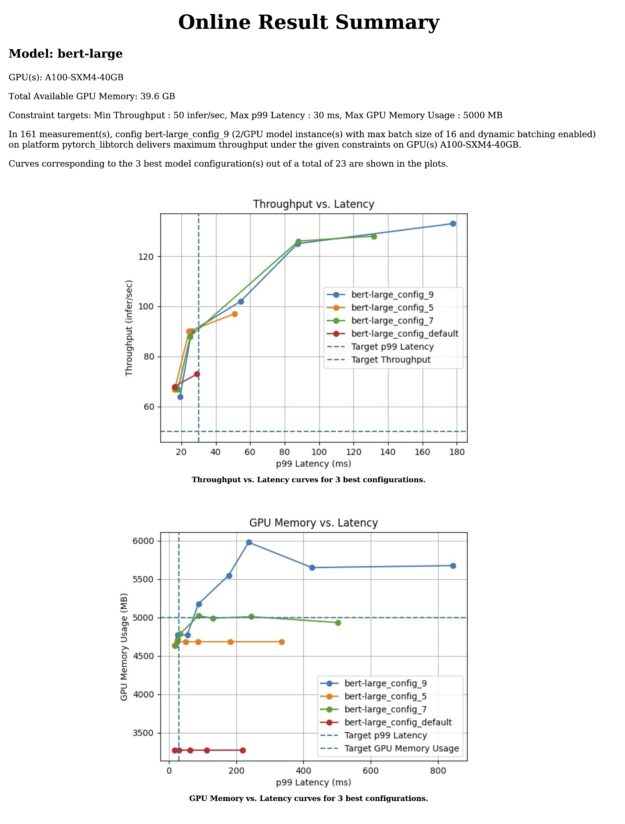
NVIDIA Triton Model Analyzer also generates plots and a more detailed report (Figure 2).
Figure 2. Sample report generated by NVIDIA Triton Model Analyzer
Summary
As enterprises find themselves serving more and more models in production, it becomes more and more difficult to make model serving decisions manually or based on heuristics. Doing this manually results in wasted development time or subpar model serving decisions, which necessitates automated tooling.
In this post, we explored how NVIDIA Triton Model Analyzer enables finding model serving configurations satisfying the application SLAs and requirements of various stakeholders. We showed how Model Analyzer can be used to sweep through various configurations, and how it can be used to satisfy specified serving constraints.
Even though we focused on a single model for this post, there are plans to have Model Analyzer perform the same analysis for multiple models at the same time. For example, you could define constraints on different models running on the same GPU and optimize each.
We hope you share our excitement about how much development time Model Analyzer will save and enable your MLOps teams to make well-informed decisions. For more information, see the /triton-inference-server/model_analyzer GitHub repo.
Using an NVIDIA Triton Inference Server, industrial manufacturer Sansera improved quality control and documentation through a custom AI pipeline.
Implementing quality control and assurance methodology in manufacturing processes and quality management systems ensures that end products meet customer requirements and satisfaction. Surface defect detection systems can use image data to perform inspections and classifications for delivering high-quality products. With advancements in AI, real-time defect detection is streamlined and automated using sensors and pretrained AI models for replicable quality control.
Sweden-based company Sansera—a producer of connecting rods for diesel engines—collaborated with AI company Aixia to implement an automated, deep learning defect detection system in their production process using computer vision.
Found in buses, trucks, and ships, every rod in the manufacturing production process must be high quality, consistent, reliable, and documented. It is imperative that the high-resolution, visual inspection system detects and classifies defects in real time.
To help Sansera reach its manufacturing process quality control goals, Aixia developed and deployed a rod inspection and detection pipeline at Sansera’s production site. At the heart of the pipeline, is an NVIDIA Triton Inference Server deployed on the NVIDIA Jetson edge AI platform and data center servers. It is implemented on an x86 server with NVIDIA A10 GPUs for inference.
Using a quality vision inspection system, robots lift and display connecting rods to a set of AI-enabled cameras. The cameras take multiple photos to capture imprints and serial numbers, which are sent through AI-based computer vision models for inspection in a controlled lighting environment. The evaluations are performed in sequence and the results provide quality control documentation. Several deep learning inferences are performed per camera view.
Figure 1. Automatic inspection of a connecting rod. A robot picks up the rod for three cameras mounted left, right, and bottom.
Each connecting rod is inspected and documented properly before release. The job of this inference workflow is to detect the imprints, inspect their quality, and provide necessary details for the product documentation. The workflow is deployed and optimized on an NVIDIA Triton Inference Server, using different frameworks and consolidates quality use cases in a streamlined fashion.
Several models, in both pre-and post-processing, are consolidated within one server instance.
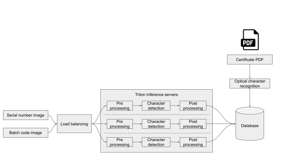
Figure 2. Scalable deployment of NVIDIA Triton inference server with here the pre-and post-processing of the image.
Using NVIDIA Triton, Aixia deploys optimized versions of the pretrained models, in the data center using high-performance GPUs, or on the edge close to the data using the Jetson edge AI platform.
Train highly accurate computer vision models with Lexset synthetic data and the NVIDIA TAO Toolkit.
To develop an accurate computer vision AI application, you need massive amounts of high-quality data. With a traditional dataset, you might spend months collecting images, getting annotations, and cleaning data. When it’s done, you could find edge cases and need more data, starting the cycle all over again.
For years, this cycle has held back AI, especially in computer vision. Lexset builds tools that enable you to generate data to solve this bottleneck. Powerful new workflows with training data can be developed and iterated as part of the AI training cycle.
Lexset’s Seahaven platform generates fully annotated datasets, including photorealistic RGB images, semantic segmentation, and depth maps, in a matter of minutes. Iteration to improve your model’s accuracy is fast and effective. It’s not a months-long process to find data for unusual events or rare conditions anymore. Just quickly adjust your configuration and generate new data to make your model better than ever.
The synthetic data generated from Seahaven can be used to fine-tune and customize pretrained models from the NVIDIA TAO Toolkit. The TAO Toolkit, a low-code AI model development solution, abstracts the complexity of AI frameworks and enables you to create custom, production-ready models for your specific use case with transfer learning.
Reduce time and increase accuracy significantly by using both Seahaven and TAO Toolkit in creating an initial dataset. Most importantly, you can use synthetic data to quickly adapt a model to changing conditions and increased complexity.
Solution overview
For this experiment, you take a simple use case and build a computer vision model capable of finding and differentiating between a common hardware item, such as screws. You start with a simple background and introduce more complexity to show how adaptable synthetic data is to changing conditions.
We created a dataset containing images with annotations of the four screws and used the TAO Toolkit Object Detection model to get started. We used Faster R-CNN, RetinaNet, and YOLOv3.
In this post, I cover the steps required to run this sample dataset, which you can download, through Faster R-CNN. To run RetinaNet or YOLOv3, the steps are the same and are in the provided Jupyter notebook.
I also share how the Lexset synthetic data can be used in concert with model training to quickly address accuracy issues that may arise as use cases become more complex.
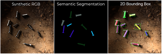
Figure 1. Synthetic screws generated by Lexset in RGB, Semantic Segmentation, and with 2D Bounding boxes.
To reproduce the results described, follow these main steps:
Use a pretrained ResNet-18 model and train a ResNet-18 Faster RCNN model on Lexset’s four screws synthetic dataset.
Use the best trained weights on the synthetic dataset and fine-tune them with 10% of the real-world four-screw dataset.
Evaluate the best trained and fine-tuned weights on the real screws validation dataset.
Run inference on the trained model.
Prerequisites
NVIDIA TAO Toolkit requires an NVIDIA GPU (for example, A100) and driver to use their Docker container, so you must have one to proceed.
You also need at least 16 GBs physical RAM, 50 GB of available memory, and an 8-Core. We tested on Python 3.6.9 and used Ubuntu 18.04. TAO Toolkit requires NVIDIA driver 455.xx or later.
The tao-launcher is strictly a python3-only package, capable of running on Python 3.6.9 or 3.7 or 3.8.
You must have an NGC account and an API key associated with your account. For more information about creating an NGC account and obtaining an API key, see the Installation Prerequisites section.
Download the dataset
Download the dataset from the Google Drive folder (link also provided in the notebook), which contains all the zip files for synthetic and real images of screws.
Extract the dataset inside synthetic_dataset_without_complex_phase1.zip and real_dataset.zip into the /data directory. The dataset directory structure should look like the following:
The code example generates the global ~/.tao_mounts.json file at the Ubuntu home directory.
Processing the dataset into TFRecords
When the dataset is downloaded and placed in a data directory, the next step is to convert the KITTI files into the TFRecord format used by NVIDIA TAO Toolkit. Generate TFrecords for both the synthetic and real datasets. This code example from the Jupyter notebook generates TFrecords:
The same conversion is applied on the real dataset by the next code example in the notebook.
Download the ResNet-18 convolutional backbone
On the setup of NGC CLI locally, download the convolutional backbone, ResNet-18.
!ngc registry model list nvidia/tao/pretrained_object_detection*
Run a benchmark experiment using synthetic data
The following commands start the training on synthetic data and all the logs are saved on out_resnet18_synth_amp16.log file. To see the logs, open the file or refresh the tab if the file was already opened.
Alternatively, you can use the tail command to see the last few lines of the logs.
!tail -f ./out_resnet18_synth_amp16.log
After the training is completed on the synthetic dataset, you can evaluate the synthetically trained model on 10% synthetic validation dataset using the following commands:
You also see the individual mAP scores for each class.
Fine-tuning the synthetic-trained model with real data
Now, use the best trained weights from synthetic training and perform the fine-tuning on 10% of the real-world screw dataset. The /train folder inside real_train is already at a 10% split and you can start the fine-tuning using the following commands:
Fine tuning on just 10% of the real-world screw dataset improves the results quickly and the mAP score above 98%. The features learned from the synthetic dataset helped during the fine-tuning on just 10% of the real-world screw dataset.
Add a complex background in the synthetic screws validation dataset
To further validate the synthetically trained model, we added 300 more images to the complex background dataset. As the initial synthetic dataset was not taken with a complex background, the mean average precision drops significantly.
Just like the real world, as the use case becomes more complex, the accuracy suffers. When validated on images containing more complex or adversarial backgrounds, the mAP score dropped from around 98% to 83.5%.
Retrain the synthetic dataset with complex backgrounds
This is where synthetic data really shines. To mitigate the loss in mAP when validated on complex images, I generated additional images with more complex backgrounds to add to the training data. I just adjusted the backgrounds so that the new training data set was ready in a manner of seconds. After being introduced, the new dataset boosted performance by an incredible 10-12% with no additional changes.
The dataset with the complex backgrounds is inside the zip file synthetic_dataset_with_complex.zip mentioned earlier. Extract this file and replace the folders inside the /data directory with the same names to have an updated synthetic dataset with a complex background.
Average Mean Precision:
mAP= 94.97%

Increase in mAP score: 11.47%
Specifically, the accuracy of the system with complex backgrounds rose as much as 11.47%, to 94.97%, after just a few minutes of work.
Conclusion
The results showed just how effective and quick it is to iterate with synthetic data and the TAO Toolkit. Using Lexset’s Seahaven, you can generate new data in a matter of minutes and use it to resolve the accuracy issues encountered with introduced complex backgrounds.
The importance of the synthetic dataset is now clear, as the performance of the fine-tuned model on the 90% validation dataset for real-world screw data is extremely good. Use a synthetic dataset for initial feature learning when you have less actual or real-world data. Synthetic datasets can save significant time and cost while producing superior results.
I believe this is the future of computer vision development, where data production occurs in tandem with model iteration. This will give greater controls to the user and enabling you to build the best systems the world has ever seen.

 Users can now produce 3D virtual worlds at human scale with the new Omniverse XR App available in beta from the NVIDIA Omniverse launcher.
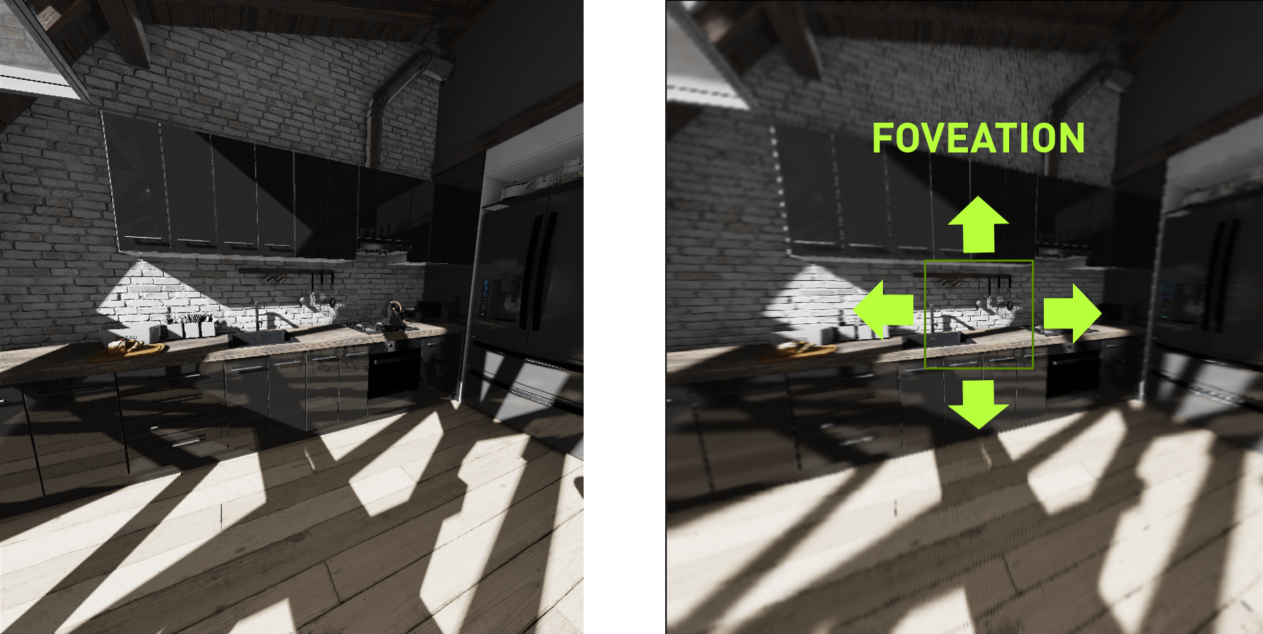
 This post presents an overview of NVIDIA Triton Model Analyzer and how it can be used to find the optimal AI model-serving configuration to satisfy application requirements.
 Using an NVIDIA Triton Inference Server, industrial manufacturer Sansera improved quality control and documentation through a custom AI pipeline.
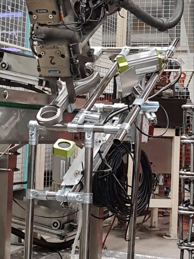
 Train highly accurate computer vision models with Lexset synthetic data and the NVIDIA TAO Toolkit.