The world’s largest democracy is poised to transform itself and the world, embracing AI on an enormous scale. Speaking with the press Friday in Bengaluru, in the context of announcements from two of India’s largest conglomerates, Reliance Industries Limited and Tata Group, NVIDIA founder and CEO Jensen Huang detailed plans to bring AI technology and Read article >
Large language models offer incredible new capabilities, expanding the frontier of what is possible with AI. But their large size and unique execution…
Large language models offer incredible new capabilities, expanding the frontier of what is possible with AI. But their large size and unique execution characteristics can make them difficult to use in cost-effective ways.
Those innovations have been integrated into the open-source NVIDIA TensorRT-LLM software, set for release in the coming weeks. TensorRT-LLM consists of the TensorRT deep learning compiler and includes optimized kernels, pre- and post-processing steps, and multi-GPU/multi-node communication primitives for groundbreaking performance on NVIDIA GPUs. It enables developers to experiment with new LLMs, offering peak performance and quick customization capabilities, without requiring deep knowledge of C++ or NVIDIA CUDA.
TensorRT-LLM improves ease of use and extensibility through an open-source modular Python API for defining, optimizing, and executing new architectures and enhancements as LLMs evolve, and can be customized easily.
For example, MosaicML has added specific features that it needs on top of TensorRT-LLM seamlessly and integrated them into their inference serving. Naveen Rao, vice president of engineering at Databricks notes that “it has been an absolute breeze.”
“TensorRT-LLM is easy to use, feature-packed with streaming of tokens, in-flight batching, paged-attention, quantization, and more, and is efficient,” Rao said. “It delivers state-of-the-art performance for LLM serving using NVIDIA GPUs and allows us to pass on the cost savings to our customers.”
Performance comparison
Summarizing articles is just one of the many applications of LLMs. The following benchmarks show performance improvements brought by TensorRT-LLM on the latest NVIDIA Hopper architecture.
The following figures reflect article summarization using an NVIDIA A100 and NVIDIA H100 with CNN/Daily Mail, a well-known dataset for evaluating summarization performance.
In Figure 1, H100 alone is 4x faster than A100. Adding TensorRT-LLM and its benefits, including in-flight batching, result in an 8X total increase to deliver the highest throughput.
Figure 1. GPT-J-6B A100 compared to H100 with and without TensorRT-LLM
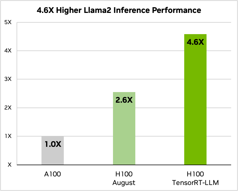
On Llama 2—a popular language model released recently by Meta and used widely by organizations looking to incorporate generative AI—TensorRT-LLM can accelerate inference performance by 4.6x compared to A100 GPUs.
Figure 2. Llama 2 70B, A100 compared to H100 with and without TensorRT-LLM
The ecosystem is innovating rapidly, developing new and diverse model architectures. Larger models unleash new capabilities and use cases. Some of the largest, most advanced language models, like Meta’s 70-billion-parameter Llama 2, require multiple GPUs working in concert to deliver responses in real time. Previously, developers looking to achieve the best performance for LLM inference had to rewrite and manually split the AI model into fragments and coordinate execution across GPUs.
TensorRT-LLM uses tensor parallelism, a type of model parallelism in which individual weight matrices are split across devices. This enables efficient inference at scale–with each model running in parallel across multiple GPUs connected through NVLink and across multiple servers–without developer intervention or model changes.
As new models and model architectures are introduced, developers can optimize their models with the latest NVIDIA AI kernels available open source in TensorRT-LLM. The supported kernel fusions include cutting-edge implementations of FlashAttention and masked multi-head attention for the context and generation phases of GPT model execution, along with many others.
Additionally, TensorRT-LLM includes fully optimized, ready-to-run versions of many LLMs widely used in production today. This includes Meta Llama 2, OpenAI GPT-2 and GPT-3, Falcon, Mosaic MPT, BLOOM, and a dozen others, all of which can be implemented with the simple-to-use TensorRT-LLM Python API.
These capabilities help developers create customized LLMs faster and more accurately to meet the needs of virtually any industry.
In-flight batching
Today’s large language models are extremely versatile. A single model can be used simultaneously for a variety of tasks that look very different from one another. From a simple question-and-answer response in a chatbot to the summarization of a document or the generation of a long chunk of code, workloads are highly dynamic, with outputs varying in size by several orders of magnitude.
This versatility can make it difficult to batch requests and execute them in parallel effectively—a common optimization for serving neural networks—which could result in some requests finishing much earlier than others.
To manage these dynamic loads, TensorRT-LLM includes an optimized scheduling technique called in-flight batching. This takes advantage of the fact that the overall text generation process for an LLM can be broken down into multiple iterations of execution on the model.
With in-flight batching, rather than waiting for the whole batch to finish before moving on to the next set of requests, the TensorRT-LLM runtime immediately evicts finished sequences from the batch. It then begins executing new requests while other requests are still in flight. In-flight batching and the additional kernel-level optimizations enable improved GPU usage and minimally double the throughput on a benchmark of real-world LLM requests on H100 Tensor Core GPUs, helping to minimize TCO.
H100 Transformer Engine with FP8
LLMs contain billions of model weights and activations, typically trained and represented with 16-bit floating point (FP16 or BF16) values where each value occupies 16 bits of memory. At inference time, however, most models can be effectively represented at lower precision, like 8-bit or even 4-bit integers (INT8 or INT4), using modern quantization techniques.
Quantization is the process of reducing the precision of a model’s weights and activations without sacrificing accuracy. Using lower precision means that each parameter is smaller, and the model takes up less space in GPU memory. This enables inference on larger models with the same hardware while spending less time on memory operations during execution.
NVIDIA H100 GPUs with TensorRT-LLM give users the ability to convert their model weights into a new FP8 format easily and compile their models to take advantage of optimized FP8 kernels automatically. This is made possible through Hopper Transformer Engine technology and done without having to change any model code.
The FP8 data format introduced by the H100 enables developers to quantize their models and radically reduce memory consumption without degrading model accuracy. FP8 quantization retains higher accuracy compared to other data formats like INT8 or INT4 while achieving the fastest performance and offering the simplest implementation.
Summary
LLMs are advancing rapidly. Diverse model architectures are being developed daily and contribute to a growing ecosystem. In turn, larger models unleash new capabilities and use cases, driving adoption across all industries.
LLM inference is reshaping the data center. Higher performance with increased accuracy yields better TCO for enterprises. Model innovations enable better customer experiences, translating into higher revenue and earnings.
When planning inference deployment projects, there are still many other considerations to achieve peak performance using state-of-the-art LLMs. Optimization rarely happens automatically. Users must consider fine-tuning factors such as parallelism, end-to-end pipelines, and advanced scheduling techniques. And they require a computing platform that can handle mixed precision without diminishing accuracy.
TensorRT-LLM comprises TensorRT’s Deep Learning Compiler, optimized kernels, pre- and post-processing, and multi-GPU/multi-node communication in a simple, open-source Python API for defining, optimizing, and executing LLMs for inference in production.
Get started with TensorRT-LLM
NVIDIA TensorRT-LLM is now available in early access and soon will be integrated into the NVIDIA NeMo framework—part of NVIDIA AI Enterprise, an enterprise-grade AI software platform with security, stability, manageability, and support. Developers and researchers will be able to access TensorRT-LLM through the NeMo framework on NGC or through the source repository on GitHub.
Note that you must be registered in the NVIDIA Developer Program to apply for the early access release. You must also be logged in using your organization’s email address. We cannot accept applications from accounts using Gmail, Yahoo, QQ, or other personal email accounts.
To participate, fill out the short application form and provide details about your use case.
NVIDIA today announced an extensive collaboration with Tata Group to deliver AI computing infrastructure and platforms for developing AI solutions. The collaboration will bring state-of-the-art AI capabilities within reach to thousands of organizations, businesses and AI researchers, and hundreds of startups in India.
In a major step to support India’s industrial sector, NVIDIA and Reliance Industries today announced a collaboration to develop India’s own foundation large language model trained on the nation’s diverse languages and tailored for generative AI applications to serve the world’s most populous nation.
Posted by Shantanu Shahane, Software Engineer, and Matthias Ihme, Research Scientist, Athena Team
Turbulence is ubiquitous in environmental and engineering fluid flows, and is encountered routinely in everyday life. A better understanding of these turbulent processes could provide valuable insights across a variety of research areas — improving the prediction of cloud formation by atmospheric transport and the spreading of wildfires by turbulent energy exchange, understanding sedimentation of deposits in rivers, and improving the efficiency of combustion in aircraft engines to reduce emissions, to name a few. However, despite its importance, our current understanding and our ability to reliably predict such flows remains limited. This is mainly attributed to the highly chaotic nature and the enormous spatial and temporal scales these fluid flows occupy, ranging from energetic, large-scale movements on the order of several meters on the high-end, where energy is injected into the fluid flow, all the way down to micrometers (μm) on the low-end, where the turbulence is dissipated into heat by viscous friction.
A powerful tool to understand these turbulent flows is the direct numerical simulation (DNS), which provides a detailed representation of the unsteady three-dimensional flow-field without making any approximations or simplifications. More specifically, this approach utilizes a discrete grid with small enough grid spacing to capture the underlying continuous equations that govern the dynamics of the system (in this case, variable-density Navier-Stokes equations, which govern all fluid flow dynamics). When the grid spacing is small enough, the discrete grid points are enough to represent the true (continuous) equations without the loss of accuracy. While this is attractive, such simulations require tremendous computational resources in order to capture the correct fluid-flow behaviors across such a wide range of spatial scales.
The actual span in spatial resolution to which direct numerical calculations must be applied depends on the task and is determined by the Reynolds number, which compares inertial to viscous forces. Typically, the Reynolds number can range between 102 up to 107 (even larger for atmospheric or interstellar problems). In 3D, the grid size for the resolution required scales roughly with the Reynolds number to the power of 4.5! Because of this strong scaling dependency, simulating such flows is generally limited to flow regimes with moderate Reynolds numbers, and typically requires access to high-performance computing systems with millions of CPU/GPU cores.
In “A TensorFlow simulation framework for scientific computing of fluid flows on tensor processing units”, we introduce a new simulation framework that enables the computation of fluid flows with TPUs. By leveraging latest advances on TensorFlow software and TPU-hardware architecture, this software tool allows detailed large-scale simulations of turbulent flows at unprecedented scale, pushing the boundaries of scientific discovery and turbulence analysis. We demonstrate that this framework scales efficiently to accommodate the scale of the problem or, alternatively, improved run times, which is remarkable since most large-scale distributed computation frameworks exhibit reduced efficiency with scaling. The software is available as an open-source project on GitHub.
Large-scale scientific computation with accelerators
The software solves variable-density Navier-Stokes equations on TPU architectures using the TensorFlow framework. The single-instruction, multiple-data (SIMD) approach is adopted for parallelization of the TPU solver implementation. The finite difference operators on a colocated structured mesh are cast as filters of the convolution function of TensorFlow, leveraging TPU’s matrix multiply unit (MXU). The framework takes advantage of the low-latency high-bandwidth inter-chips interconnect (ICI) between the TPU accelerators. In addition, by leveraging the single-precision floating-point computations and highly optimized executable through the accelerated linear algebra (XLA) compiler, it’s possible to perform large-scale simulations with excellent scaling on TPU hardware architectures.
This research effort demonstrates that the graph-based TensorFlow in combination with new types of ML special purpose hardware, can be used as a programming paradigm to solve partial differential equations representing multiphysics flows. The latter is achieved by augmenting the Navier-Stokes equations with physical models to account for chemical reactions, heat-transfer, and density changes to enable, for example, simulations of cloud formation and wildfires.
It’s worth noting that this framework is the first open-source computational fluid dynamics (CFD) framework for high-performance, large-scale simulations to fully leverage the cloud accelerators that have become common (and become a commodity) with the advancement of machine learning (ML) in recent years. While our work focuses on using TPU accelerators, the code can be easily adjusted for other accelerators, such as GPU clusters.
This framework demonstrates a way to greatly reduce the cost and turn-around time associated with running large-scale scientific CFD simulations and enables even greater iteration speed in fields, such as climate and weather research. Since the framework is implemented using TensorFlow, an ML language, it also enables the ready integration with ML methods and allows the exploration of ML approaches on CFD problems. With the general accessibility of TPU and GPU hardware, this approach lowers the barrier for researchers to contribute to our understanding of large-scale turbulent systems.
Framework validation and homogeneous isotropic turbulence
Beyond demonstrating the performance and the scaling capabilities, it is also critical to validate the correctness of this framework to ensure that when it is used for CFD problems, we get reasonable results. For this purpose, researchers typically use idealized benchmark problems during CFD solver development, many of which we adopted in our work (more details in the paper).
One such benchmark for turbulence analysis is homogeneous isotropic turbulence(HIT), which is a canonical and well studied flow in which the statistical properties, such as kinetic energy, are invariant under translations and rotations of the coordinate axes. By pushing the resolution to the limits of the current state of the art, we were able to perform direct numerical simulations with more than eight billion degrees of freedom — equivalent to a three-dimensional mesh with 2,048 grid points along each of the three directions. We used 512 TPU-v4 cores, distributing the computation of the grid points along the x, y, and z axes to a distribution of [2,2,128] cores, respectively, optimized for the performance on TPU. The wall clock time per timestep was around 425 milliseconds and the flow was simulated for a total of 400,000 timesteps. 50 TB data, which includes the velocity and density fields, is stored for 400 timesteps (every 1,000th step). To our knowledge, this is one of the largest turbulent flow simulations of its kind conducted to date.
Due to the complex, chaotic nature of the turbulent flow field, which extends across several magnitudes of resolution, simulating the system in high resolution is necessary. Because we employ a fine-resolution grid with eight billion points, we are able to accurately resolve the field.
Contours of x-component of velocity along the z midplane. The high resolution of the simulation is critical to accurately represent the turbulent field.
The turbulent kinetic energy and dissipation rates are two statistical quantities commonly used to analyze a turbulent flow. The temporal decay of these properties in a turbulent field without additional energy injection is due to viscous dissipation and the decay asymptotes follow the expected analytical power law. This is in agreement with the theoretical asymptotes and observations reported in the literature and thus, validates our framework.
Solid line: Temporal evolution of turbulent kinetic energy (k). Dashed line: Analytical power laws for decaying homogeneous isotropic turbulence (n=1.3) (Ⲧl: eddy turnover time).
Solid line: Temporal evolution of dissipation rate (ε). Dashed line: Analytical power laws for decaying homogeneous isotropic turbulence (n=1.3).
The energy spectrum of a turbulent flow represents the energy content across wavenumber, where the wavenumber k is proportional to the inverse wavelength λ (i.e., k ∝ 1/λ). Generally, the spectrum can be qualitatively divided into three ranges: source range, inertial range and viscous dissipative range (from left to right on the wavenumber axis, below). The lowest wavenumbers in the source range correspond to the largest turbulent eddies, which have the most energy content. These large eddies transfer energy to turbulence in the intermediate wavenumbers (inertial range), which is statistically isotropic (i.e., essentially uniform in all directions). The smallest eddies, corresponding to the largest wavenumbers, are dissipated into thermal energy by the viscosity of the fluid. By virtue of the fine grid having 2,048 points in each of the three spatial directions, we are able to resolve the flow field up to the length scale at which viscous dissipation takes place. This direct numerical simulation approach is the most accurate as it does not require any closure model to approximate the energy cascade below the grid size.
Spectrum of turbulent kinetic energy at different time instances. The spectrum is normalized by the instantaneous integral length (l) and the turbulent kinetic energy (k).
A new era for turbulent flows research
More recently, we extended this framework to predict wildfires and atmospheric flows, which is relevant for climate-risk assessment. Apart from enabling high-fidelity simulations of complex turbulent flows, this simulation framework also provides capabilities for scientific machine learning (SciML) — for example, downsampling from a fine to a coarse grid (model reduction) or building models that run at lower resolution while still capturing the correct dynamic behaviors. It could also provide avenues for further scientific discovery, such as building ML-based models to better parameterize microphysics of turbulent flows, including physical relationships between temperature, pressure, vapor fraction, etc., and could improve upon various control tasks, e.g., to reduce the energy consumption of buildings or find more efficient propeller shapes. While attractive, a main bottleneck in SciML has been the availability of data for training. To explore this, we have been working with groups at Stanford and Kaggle to make the data from our high-resolution HIT simulation available through a community-hosted web-platform, BLASTNet, to provide broad access to high-fidelity data to the research community via a network-of-datasets approach. We hope that the availability of these emerging high-fidelity simulation tools in conjunction with community-driven datasets will lead to significant advances in various areas of fluid mechanics.
Acknowledgements
We would like to thank Qing Wang, Yi-Fan Chen, and John Anderson for consulting and advice, Tyler Russell and Carla Bromberg for program management.
Thanks to rapid technological advances, consumers have become accustomed to an unprecedented level of convenience and efficiency. Smartphones make it easier than ever to search for a product and have it delivered right to the front door. Video chat technology lets friends and family on different continents connect with ease. With voice command tools, AI Read article >
NVIDIA has already made available a GPU driver binary symbols server for Windows. Now, NVIDIA is making available a repository of CUDA Toolkit symbols for…
NVIDIA is introducing CUDA Toolkit symbols for Linux for an application development enhancement. During application development, you can now download obfuscated symbols for NVIDIA libraries that are being debugged or profiled in your application. This is shipping initially for the CUDA Driver (libcuda.so) and the CUDA Runtime (libcudart.so), with more libraries to be added.
For instance, when an issue appears to relate to a CUDA API, it may not always be possible to provide NVIDIA with a reproducing example, core dump, or unsymbolized stack traces with all library load information. Providing a symbolized call stack can help speed up the debug process.
We are only hosting symbol files, so debug data will not be distributed. The symbol files contain obfuscated symbol names.
Quickstart guide
There are two recommended ways to use the obfuscated symbols for each library:
By unstripping the library
By deploying the .sym file as a symbol file for the library
# Determine the symbol file to fetch and obtain it
$ readelf -n /usr/local/cuda/lib64/libcudart.so

# ... Build ID: 70f26eb93e24216ffc0e93ccd8da31612d277030
# Browse to https://cudatoolkit-symbols.nvidia.com/libcudart.so/70f26eb93e24216ffc0e93ccd8da31612d277030/index.html to determine filename to download
$ wget https://cudatoolkit-symbols.nvidia.com/libcudart.so/70f26eb93e24216ffc0e93ccd8da31612d277030/libcudart.so.12.2.128.sym

# Then with appropriate permissions, either unstrip,
$ eu-unstrip /usr/local/cuda-12.2/targets/x86_64-linux/lib/libcudart.so.12.2.128 libcudart.so.12.2.128.sym –o /usr/local/cuda-12.2/targets/x86_64-linux/lib/libcudart.so.12.2.128

# Or, with appropriate permissions, deploy as symbol file
# By splitting the Build ID into first two characters as directory, then remaining with ".debug" extension
$ cp libcudart.so.12.2.128.sym /usr/lib/debug/.build-id/70/f26eb93e24216ffc0e93ccd8da31612d277030.debug
Example: Symbolizing
Here is a simplified example to show the uses of symbolizing. The sample application test_shared has a data corruption that leads to an invalid handle being passed to the CUDA Runtime API cudaStreamDestroy. With a default install of CUDA Toolkit and no obfuscated symbols, the output in gdb might look like the following:
Thread 1 "test_shared" received signal SIGSEGV, Segmentation fault.
0x00007ffff65f9468 in ?? () from /lib/x86_64-linux-gnu/libcuda.so.1
(gdb) bt
#0  0x00007ffff65f9468 in ?? () from /lib/x86_64-linux-gnu/libcuda.so.1
#1  0x00007ffff6657e1f in ?? () from /lib/x86_64-linux-gnu/libcuda.so.1
#2  0x00007ffff6013845 in ?? () from /usr/local/cuda/lib64/libcudart.so.12
#3  0x00007ffff604e698 in cudaStreamDestroy () from /usr/local/cuda/lib64/libcudart.so.12
#4  0x00005555555554e3 in main ()
After applying the obfuscated symbols in one of the ways described earlier, it would give a stack trace like the following example:
Thread 1 "test_shared" received signal SIGSEGV, Segmentation fault.
0x00007ffff65f9468 in libcuda_8e2eae48ba8eb68460582f76460557784d48a71a () from /lib/x86_64-linux-gnu/libcuda.so.1
(gdb) bt
#0  0x00007ffff65f9468 in libcuda_8e2eae48ba8eb68460582f76460557784d48a71a () from /lib/x86_64-linux-gnu/libcuda.so.1
#1  0x00007ffff6657e1f in libcuda_10c0735c5053f532d0a8bdb0959e754c2e7a4e3d () from /lib/x86_64-linux-gnu/libcuda.so.1
#2  0x00007ffff6013845 in libcudart_43d9a0d553511aed66b6c644856e24b360d81d0c () from /usr/local/cuda/lib64/libcudart.so.12
#3  0x00007ffff604e698 in cudaStreamDestroy () from /usr/local/cuda/lib64/libcudart.so.12
#4  0x00005555555554e3 in main ()
The symbolized call stack can then be documented as part of the bug description provided to NVIDIA for analysis.
Conclusion
When you have to profile and debug applications using CUDA and want to share a call stack with NVIDIA for analysis, use the CUDA symbol server. Profiling and debugging will be faster and easier.
For questions or issues, dive into the forum at Developer Tools.
As data scientists, we often face the challenging task of training large models on huge datasets. One commonly used tool, XGBoost, is a robust and efficient…
As data scientists, we often face the challenging task of training large models on huge datasets. One commonly used tool, XGBoost, is a robust and efficient gradient-boosting framework that’s been widely adopted due to its speed and performance for large tabular data.
Using multiple GPUs should theoretically provide a significant boost in computational power, resulting in faster model training. Yet, many users have found it challenging when attempting to leverage this power through Dask XGBoost. Dask is a flexible open-source Python library for parallel computing and XGBoost provides Dask APIs to train CPU or GPU Dask DataFrames.
A common hurdle of training Dask XGBoost is handling out of memory (OOM) errors at different stages, including
Loading the training data
Converting the DataFrame into XGBoost’s DMatrix format
During the actual model training
Addressing these memory issues can be challenging, but very rewarding because the potential benefits of multi-GPU training are enticing.
Top takeaways
This post explores how you can optimize Dask XGBoost on multiple GPUs and manage memory errors. Training XGBoost on large datasets presents a variety of challenges. I use the Otto Group Product Classification Challenge dataset to demonstrate the OOM problem and how to fix it. The dataset has 180 million rows and 152 columns, totaling 110 GB when loaded into memory.
The key issues we tackle include:
Installation using the latest version of RAPIDS and the correct version of XGBoost.
Setting environment variables.
Dealing with OOM errors.
Utilizing UCX-py for more speedup.
Be sure to follow along with the accompanying Notebooks for each section.
Each method has unique considerations. For this guide, I recommend using Mamba, while adhering to the conda install instructions. Mamba provides similar functionalities as conda but is much faster, especially for dependency resolution. Specifically, I opted for a fresh installation of mamba.
Install the latest RAPIDS version
As a best practice, always install the latest RAPIDS libraries available to use the latest features. You can find up-to-date install instructions in the RAPIDS Installation Guide.
This post uses version 23.04, which can be installed with the following command:
This instruction installs all the libraries required including Dask, Dask-cuDF, XGBoost, and more. In particular, you’ll want to check the XGBoost library installed using the command:
mamba list xgboost
The output is listed in Table 1:
Name
Version
Build
Channel
XGBoost
1.7.1dev.rapidsai23.04
cuda_11_py310_3
rapidsai-nightly
Tabel 1. Install the correct XGBoost whose channel should be rapidsai or rapidsai-nightly
Avoid manual updates for XGBoost
Some users might notice that the version of XGBoost is not the latest, which is 1.7.5. Manually updating or installing XGBoost using pip or conda-forge is problematic when training XGBoost together with UCX.
The error message will read something like the following: Exception: “XGBoostError(‘[14:14:27] /opt/conda/conda-bld/work/rabit/include/rabit/internal/utils.h:86: Allreduce failed’)”
Instead, use the XGBoost installed from RAPIDS. A quick way to verify the correctness of the XGBoost version is mamba list xgboost and check the “channel” of the xgboost, which should be “rapidsai” or “rapidsai-nightly”.
XGBoost in the rapidsai channel is built with the RMM plug-in enabled and delivers the best performance regarding multi-GPU training.
Multi-GPU training walkthrough
First, I’ll walk through a multi-GPU training notebook for the Otto dataset and cover the steps to make it work. Later on, we will talk about some advanced optimizations including UCX and spilling.
You can also find the XGB-186-CLICKS-DASK Notebook on GitHub. Alternatively, we provide a python script with full command line configurability.
The main libraries we are going to use are xgboost, dask, dask_cuda, and dask-cudf.
import os

import dask

import dask_cudf

import xgboost as xgb

from dask.distributed import Client

from dask_cuda import LocalCUDACluster
Environment set up
First, let’s set our environment variables to make sure our GPUs are visible. This example uses eight GPUs with 32 GB of memory on each GPU, which is the minimum requirement to run this notebook without OOM complications. In Section Enable memory spilling below we will discuss techniques to lower this requirement to 4 GPUs.
GPUs = ','.join([str(i) for i in range(0,8)])
os.environ['CUDA_VISIBLE_DEVICES'] = GPUs
Next, define a helper function to create a local GPU cluster for a mutli-GPU single node.
The dataset consists of 152 columns that represent engineered features, providing information about the frequency with which specific product pairs are viewed or purchased together. The objective is to predict which product the user will click next based on their browsing history. The details of this dataset can be found in this writeup.
Even at this early stage, out of memory errors can occur. This issue often arises due to excessively large row groups in parquet files. To resolve this, we recommend rewriting the parquet files with smaller row groups. For a more in-depth explanation, refer to the Parquet Large Row Group Demo Notebook.
After loading the data, we can check its shape and memory usage.
The ‘clicks’ column is our target, which means if the recommended item was clicked by the user. We ignore the ID columns and use the rest columns as features.
FEATURES = users.columns[2:]

TARS = ['clicks']

FEATURES = [f for f in FEATURES if f not in TARS]
Next, we create a DaskQuantileDMatrix which is the input data format for training xgboost models. DaskQuantileDMatrix is a drop-in replacement for the DaskDMatrix when the histogram tree method is used. It helps reduce overall memory usage.
This step is critical to avoid OOM errors. If we use the DaskDMatrix OOM occurs even with 16 GPUs. In contrast, DaskQuantileDMatrix enables training xgboot with eight GPUs or less without OOM errors.
We then set our XGBoost model parameters and start the training process. Given the target column ‘clicks’ is binary, we use the binary classification objective.
Now, you’re ready to train the XGBoost model using all eight GPUs.
Output:
[99] train-map:0.20168

CPU times: user 7.45 s, sys: 1.93 s, total: 9.38 s

Wall time: 1min 10s
That’s it! You’re done with training the XGBoost model using multiple GPUs.
Enable memory spilling
In the previous XGB-186-CLICKS-DASK Notebook, training the XGBoost model on the Otto dataset required a minimum of eight GPUs. Given that this dataset occupies 110GB in memory, and each V100 GPU offers 32GB, the data-to-GPU-memory ratio amounts to a mere 43% (calculated as 110/(32*8)).
Optimally, we’d halve this by using just four GPUs. Yet, a straightforward reduction of GPUs in our previous setup invariably leads to OOM errors. This issue arises from the creation of temporary variables needed to generate the DaskQuantileDMatrix from the Dask cuDF dataframe and in other steps of training XGBoost. These variables themselves consume a substantial share of the GPU memory.
Optimize the same GPU resources to train larger datasets
In the XGB-186-CLICKS-DASK-SPILL Notebook, I introduce minor tweaks to the previous setup. By enabling spilling, you can now train on the same dataset using just four GPUs. This technique allows you to train much larger data with the same GPU resources.
Spilling is the technique that moves data automatically when an operation that would otherwise succeed runs out of memory due to other dataframes or series taking up needed space in GPU memory. It enables out-of-core computations on datasets that don’t fit into memory. RAPIDS cuDF and dask-cudf now support spilling from GPU to CPU memory
Enabling spilling is surprisingly easy, where we just need to reconfigure the cluster with two new parameters, device_memory_limit and jit_unspill:
device_memory_limit='10GB’ sets a limit on the amount of GPU memory that can be used by each GPU before spilling is triggered. Our configuration intentionally assigns a device_memory_limit of 10GB, substantially less than the total 32GB of the GPU. This is a deliberate strategy designed to preempt OOM errors during XGBoost training.
It’s also important to understand that memory usage by XGBoost isn’t managed directly by Dask-CUDA or Dask-cuDF. Therefore, to prevent memory overflow, Dask-CUDA and Dask-cuDF need to initiate the spilling process before the memory limit is reached by XGBoost operations.
Jit_unspill enables Just-In-Time un-spilling, which means that the cluster will automatically spill data from GPU memory to main memory when GPU memory is running low, and unspill it back just in time for a computation.
And that’s it! The rest of the notebook is identical to the previous notebook. Now it can train with just four GPUs, saving 50% of computing resources.
Use Unified Communication X (UCX) for optimal data transfer
UCX-py is a high-performance communication protocol that provides optimized data transfer capabilities, which is particularly useful for GPU-to-GPU communication.
To use UCX effectively, we need to set another environment variable RAPIDS_NO_INITIALIZE:
os.environ["RAPIDS_NO_INITIALIZE"] = "1"
It stops cuDF from running various diagnostics on import which requires the creation of an NVIDIA CUDA context. When running distributed and using UCX, we have to bring up the networking stack before a CUDA context is created (for various reasons). By setting that environment variable, any child processes that import cuDF do not create a CUDA context before UCX has a chance to do so.
The protocol=’ucx’ parameter specifies UCX to be the communication protocol used for transferring data between the workers in the cluster.
Use the prmm_pool_size=’29GB’ parameter to set the size of the RAPIDS Memory Manager (RMM) pool for each worker. RMM allows for efficient use of GPU memory. In this case, the pool size is set to 29GB which is less than the total GPU memory size of 32GB. This adjustment is crucial as it accounts for the fact that XGBoost creates certain intermediate variables that exist outside the control of the RMM pool.
By simply enabling UCX, we experienced a substantial acceleration in our training times—a significant speed boost of 20% with spilling, and an impressive 40.7% speedup when spilling was not needed. Refer to the XGB-186-CLICKS-DASK-UCX-SPILL Notebook for details.
Configure local_directory
There are times when warning messages emerge, such as, “UserWarning: Creating scratch directories is taking a surprisingly long time.” This is a signal indicating that disk performance is becoming a bottleneck.
To circumvent this issue, we could set local_directory of dask-cuda, which specifies the path on the local machine to store temporary files. These temporary files are used during Dask’s spill-to-disk operations.
A recommended practice is to set the local_directory to a location on a fast storage device. For instance, we could set local_directory to /raid/dask_dir if it is on a high-speed local SSD. Making this simple change can significantly reduce the time it takes for scratch directory operations, optimizing your overall workflow.
As shown in Table 2, the two main optimization techniques are UCX and spilling. We managed to train XGBoost with just four GPUs and 128GB of memory. We will also show the performance scales nicely to more GPUs.
Spilling off
Spilling on
UCX off
135s / 8GPUs / 256 GB
270s / 4GPUs / 128 GB
UCX on
80s / 8GPUs / 256 GB
217s / 4GPUs / 128 GB
Table 2. Overview of four combinations of optimizations
In each cell, the numbers represent end-to-end execution time, the minimum number of GPUs required, and the total GPU memory available. All four demos accomplish the same task of loading and training 110 GB of Otto data.
Summary
In conclusion, leveraging Dask and XGBoost with multiple GPUs can be an exciting adventure, despite the occasional bumps like out of memory errors.
You can mitigate these memory challenges and tap into the potential of multi-GPU model training by:
Carefully configuring parameters such as row group size in the input parquet files
Ensuring the correct installation of RAPIDS and XGBoost
Utilizing Dask Quantile DMatrix
Enabling spilling
Furthermore, by applying advanced features such as UCX-Py, you can significantly speed up training times.
Sign up for the latest Data Science news. Get the latest announcements, notebooks, hands-on tutorials, events, and more in your inbox once a month from NVIDIA.

 On Sept. 19, learn how NVIDIA TAO integrates with the ClearML platform to deploy and maintain machine learning models in production environments.
 Large language models offer incredible new capabilities, expanding the frontier of what is possible with AI. But their large size and unique execution…
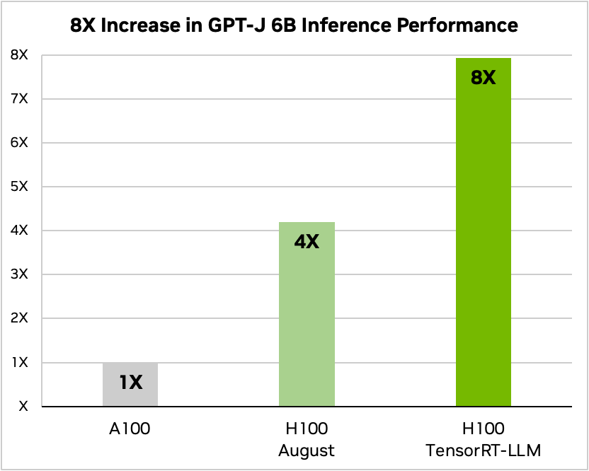
 Learn key techniques and tools required to train a deep learning model in this virtual hands-on workshop.
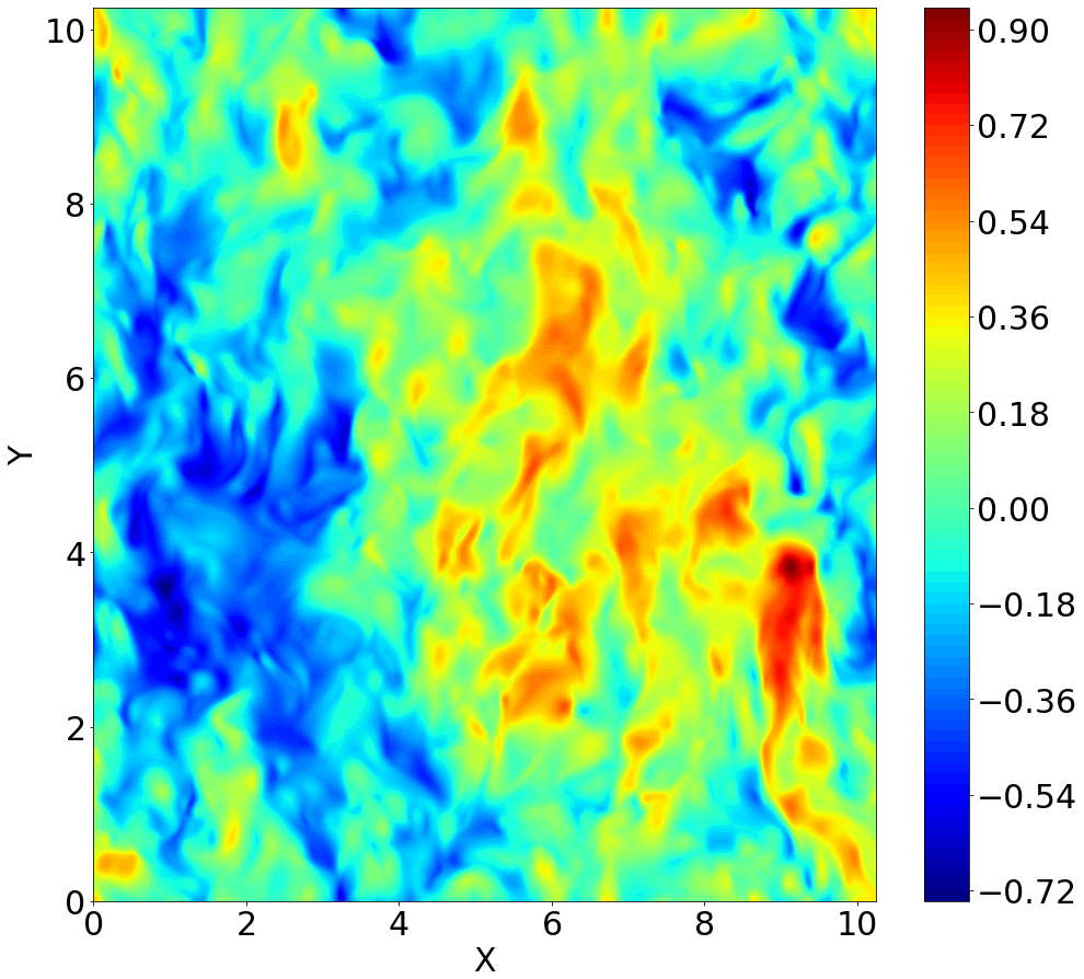


 NVIDIA has already made available a GPU driver binary symbols server for Windows. Now, NVIDIA is making available a repository of CUDA Toolkit symbols for…
 As data scientists, we often face the challenging task of training large models on huge datasets. One commonly used tool, XGBoost, is a robust and efficient…