Caching is as fundamental to computing as arrays, symbols, or strings. Various layers of caching throughout the stack hold instructions from memory while…
Caching is as fundamental to computing as arrays, symbols, or strings. Various layers of caching throughout the stack hold instructions from memory while pending on your CPU. They enable you to reload the page quickly and without re-authenticating, should you navigate away. They also dramatically decrease application workloads, and increase throughput by not re-running the same queries repeatedly.
Caching is not new to NVIDIA Triton Inference Server, which is a system tuned to answering questions in the form of running inferences on tensors. Running inferences is a relatively computationally expensive task that often calls on the same inference to run repeatedly. This naturally lends itself to using a caching pattern.
The NVIDIA Triton team recently implemented the Triton response cache using the Triton local cache library. They have also built a cache API to make this caching pattern extensible within Triton. The Redis team then leveraged that API to build the Redis cache for NVIDIA Triton.
In this post, the Redis team explores the benefits of the new Redis implementation of the Triton Caching API. We explore how to get started and discuss some of the best practices for using Redis to supercharge your NVIDIA Triton instance.
What is Redis?
Redis is an acronym for REmote DIctionary Server. It is a NoSQL database that operates as a key-value data structure store. Redis is memory-first, meaning that the entire dataset in Redis is stored in memory, and optionally persisted to disk, based on configuration. Because it is a key-value database completely held in memory, Redis is blazingly fast. Execution times are measured in microseconds, and throughputs in tens of thousands of operations a second.
The remarkable speed and typical access pattern of Redis make it ideal for caching. Redis is synonymous with caching and is consequentially one of the built-in distributed caches of most major application frameworks across a variety of developer communities.
What is local cache?
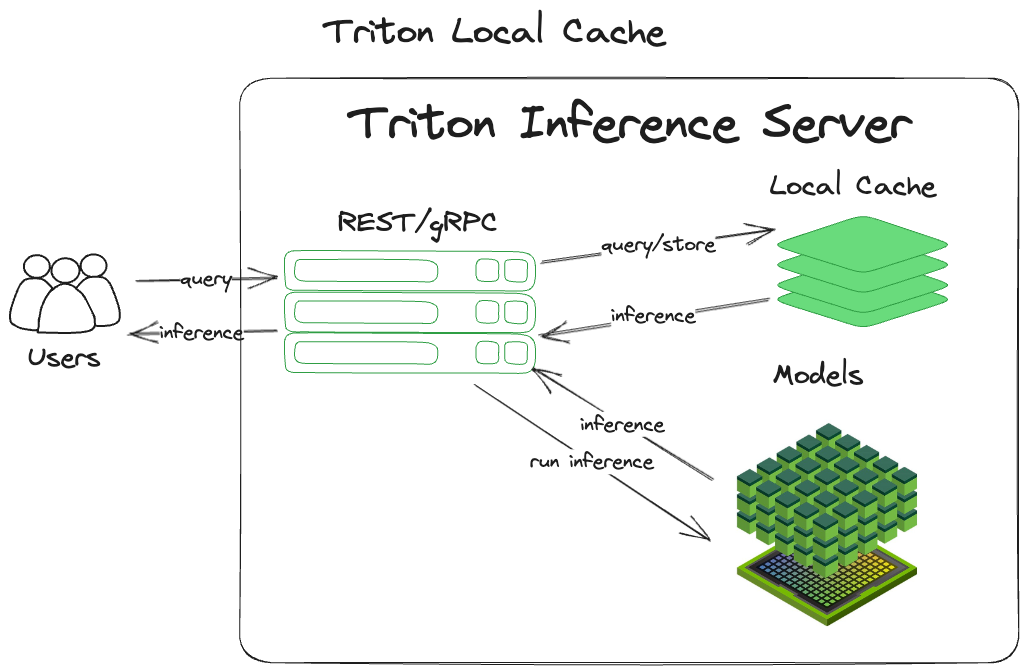
The local cache is an in-memory derivation of the most common caching pattern out there (cache-aside). It is simple and efficient, making it easy to grasp and implement. After receiving a query, NVIDIA Triton:
- Computes a hash of the input query, including the tensor and some metadata. This becomes the inference key.
- Checks for a previously inferred result for that tensor at that key.
- Returns any results found.
- Performs the inference if no results are found.
- Caches the inference in memory using the key for storage.
- Returns the inference.
‘Local’ means that it is staying local to the process and storing the cache in the system’s main memory. Figure 1 shows the implementation of this pattern.
Benefits of local cache
There are a variety of benefits that flow naturally from using this pattern. Because the queries are cached, they can be retrieved again easily without rerunning the tensor through the models. Because everything is maintained locally in the process memory, there is no need to leave the process or machine to retrieve the cached data. These two in concert can dramatically increase throughput, as well as decrease the cost of this computation.
Drawbacks of local cache
This technique does have drawbacks. Because the cache is tied directly into the process memory, each time the Triton process restarts, it starts from square one (generally referred to as a cold start). You will not see the benefits from caching while the cache warms up. Also, because the cache is process-locked, other instances of Triton will not be able to share the cache, leading to duplication of caching across each node.
The other major drawback concerns resource contention. Since the local cache is tied to the process, it is limited to the resources of the system that Triton runs on. This means that it is impossible to horizontally scale the resources allocated to the cache (distributing the cache across multiple machines), which limits the options for expanding the local cache to vertical scaling. This makes the server running Triton bigger.
Benefits of distributed caching with Redis
Unlike local caching, distributed caching leverages an external service (such as Redis) to distribute the cache off the local server. This confers several advantages to the NVIDIA Triton caching API:
- Redis is not bound to the available system resources of the same machine as Triton, or for that matter, a single machine.
- Redis is decoupled from Triton’s process life cycle, enabling multiple Triton instances to leverage the same cache.
- Redis is extremely fast (execution times are typically sub-milliseconds).
- Redis is a significantly more specialized, feature-rich, and tunable caching service compared to the Triton local cache.
- Redis provides immediate access to tried and tested high availability, horizontal scaling, and cache-eviction features out of the box.
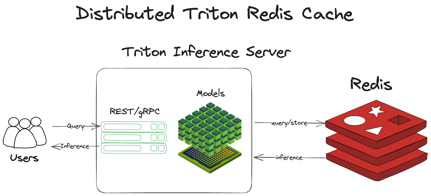
Distributed caching with Redis works much the same way as the local cache. Rather than staying within the same process, it crosses out of the Triton server process to Redis to check the cache and store inferences. After receiving a query, NVIDIA Triton:
- Computes a hash of the input query, including the tensor and some metadata. This becomes the inference key.
- Checks Redis for a previous run inference.
- Returns that inference, if it exists.
- Runs the tensor through Triton if the inference does not exist.
- Stores the inference in Redis.
- Returns the inference.
Architecturally, this is shown in Figure 2.
Distributed cache set up and configuration
To set up the distributed Redis cache requires two top-level steps:
- Deploy your Redis instance.
- Configure NVIDIA Triton to point at the Redis instance.
Triton will take care of the rest for you. To learn more about Redis, see redis.io, docs.redis.com, and Redis University.
To configure Triton to point at your Redis instance, use the --cache-config options in your start command. In the model config, enable the response cache for the model with {{response_cache { enable: true }}}.
tritonserver --cache-config redis,host=localhost --cache-config redis,port=6379The Redis cache calls on you to minimally configure the host and port of your Redis instance. For a full enumeration of configuration options, see the Triton Redis Cache GitHub repo.
Best practices with Redis
Redis is lightweight, easy to use, and extremely fast. Even with its small footprint and simplicity, there is much you can configure in and around Redis to optimize it for your use case. This section highlights best practices for using and configuring Redis.
Minimize round-trip time
The only real drawback of using an external service like Redis over an in-process memory cache is that the queries to Redis will, at least, have to cross process. They typically need to cross server boundaries as well.
Because of this, minimizing round-trip times (RTT) is of paramount importance in optimizing the use of Redis as a cache. The topic of how to minimize RTT is far too complex a topic to dive into in this post. A couple of key tips: maintain the locality of your Redis servers to your Triton servers and have them physically close to each other. If they are in a data center, try to keep them in the same rack or availability zone.
Scaling and high availability
Redis Cluster enables you to scale your Redis instances horizontally over multiple shards. The cluster includes the ability to replicate your Redis instance. If there is a failure in your primary shard, the replica can be promoted for high availability.
Maximum memory and eviction
If Redis memory is not capped, it will use all the available memory on the system that the OS will release to it. Set the maxmemory configuration key in redis.conf. But what happens if you set maxmemory and Redis runs out of memory? The default is, as you might expect, to stop accepting new writes to Redis.
However, you can also set an eviction policy. An eviction policy uses some basic intelligence to decide which keys might be good candidates to kick out of Redis. Allowing Redis to evict keys that no longer make sense to store enables it to continue accepting new writes without interruption when the memory fills.
For a full explanation of different Redis eviction policies, see key eviction in the Redis manual.
Durability and persistence
Redis is memory-first, meaning everything is stored in memory. If you do not configure persistence and the Redis process dies, it will essentially return to a cold-started state. (The cache will need to ‘warm up’ before you get the benefits from caching.)
There are two options for persisting Redis. Taking periodic snapshots of the state of Redis in .rdb files and keeping a log of all write commands in the append-only file. For a full explanation of these methods, see persistence in the Redis manual.
Speed comparison
Getting down to brass tacks, this section explores a comprehensive difference between the performance of Triton without Redis and Triton with Redis. In the interest of simplicity, we leveraged the perf_analyzer tool the Triton team built for measuring performance with Triton. We tested with two separate models, DenseNet and Simple.
We ran Triton Server version 23.06 on a Google Cloud Platform (GCP) n1-standard-4 VM with a single NVIDIA T4 GPU. We also ran a vanilla open-source Redis instance on a GCP n2-standard-4 VM. Finally, we ran the Triton client image in Docker on a GCP e2-medium VM.
We ran the perf_analyzer tool with both the DenseNet and Simple models, 10 times on each caching configuration, with no caching, with Redis as the cache, and with the local cache as the cache. We then averaged the results of these runs.
It is important to note that these runs assume a 100% cache-hit rate. So, the measurement is the difference between the performance of Triton when it has encountered the entry in the past and when it has not.
We used the following command for the DenseNet model:
perf_analyzer -m densenet_onnx -u triton-server:8000We used the following command for the Simple model:
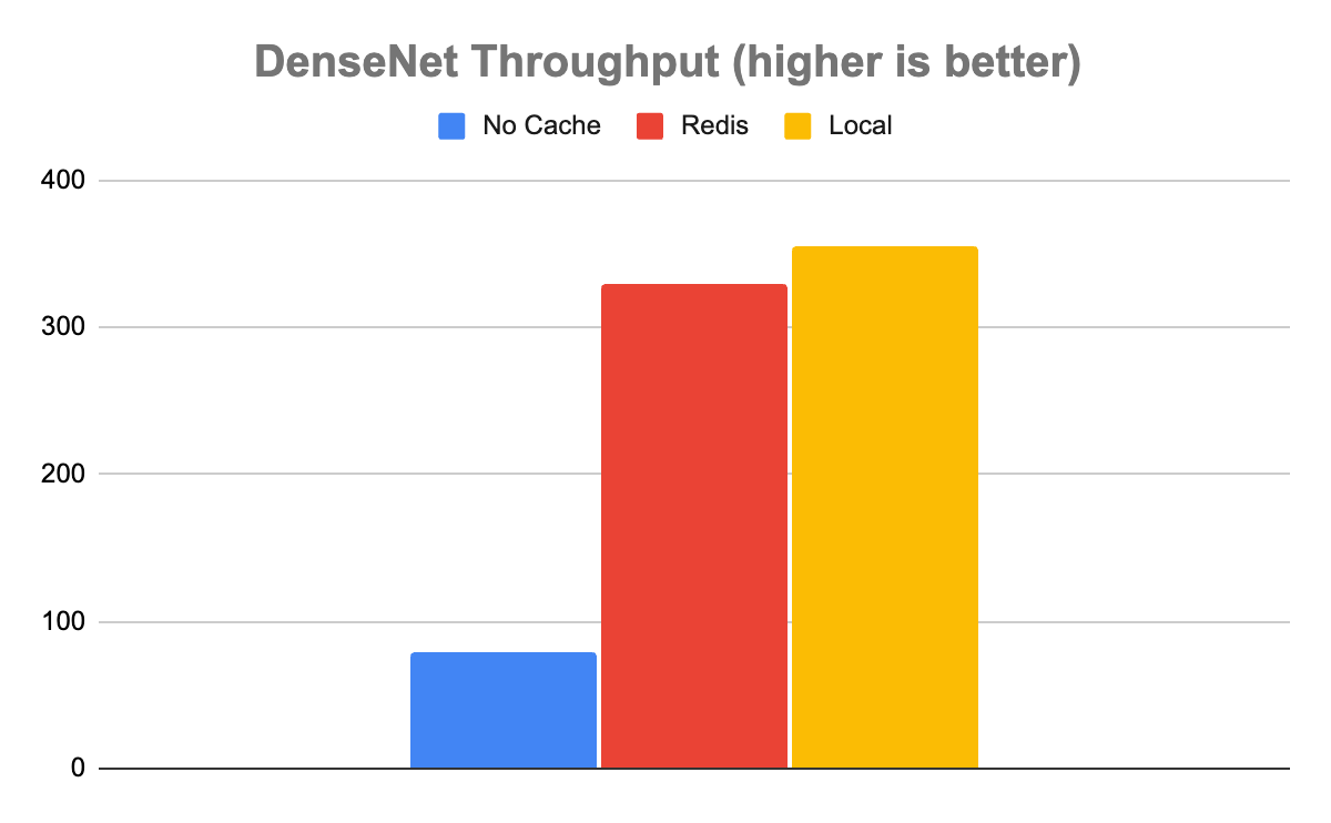
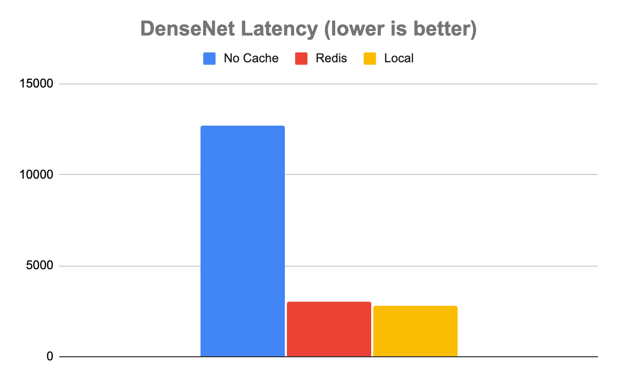
perf_analyzer -m simple -u triton-server:8000In the case of the DenseNet model, the results showed that using either cache was dramatically better than running with no cache. Without caching, Triton was able to handle 80 inferences per second (inference/sec) with an average latency of 12,680 µs. With Redis, it was about 4x faster, processing 329 inference/sec with an average latency of 3,030 µs.
Interestingly, while local caching was somewhat faster than Redis, as you would expect it to be, it was only marginally faster. Local caching resulted in a throughput of 355 inference/sec with a latency of 2,817 µs, only about 8% faster. In this case, it’s clear that the speed tradeoff of caching locally versus in Redis is a marginal one. Given all the extra benefits that come from using a distributed versus a local cache, distributed will almost certainly be the way to go when handling these kinds of data.
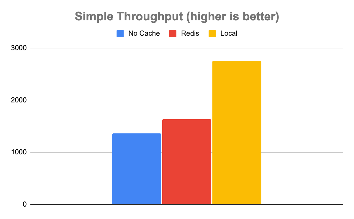
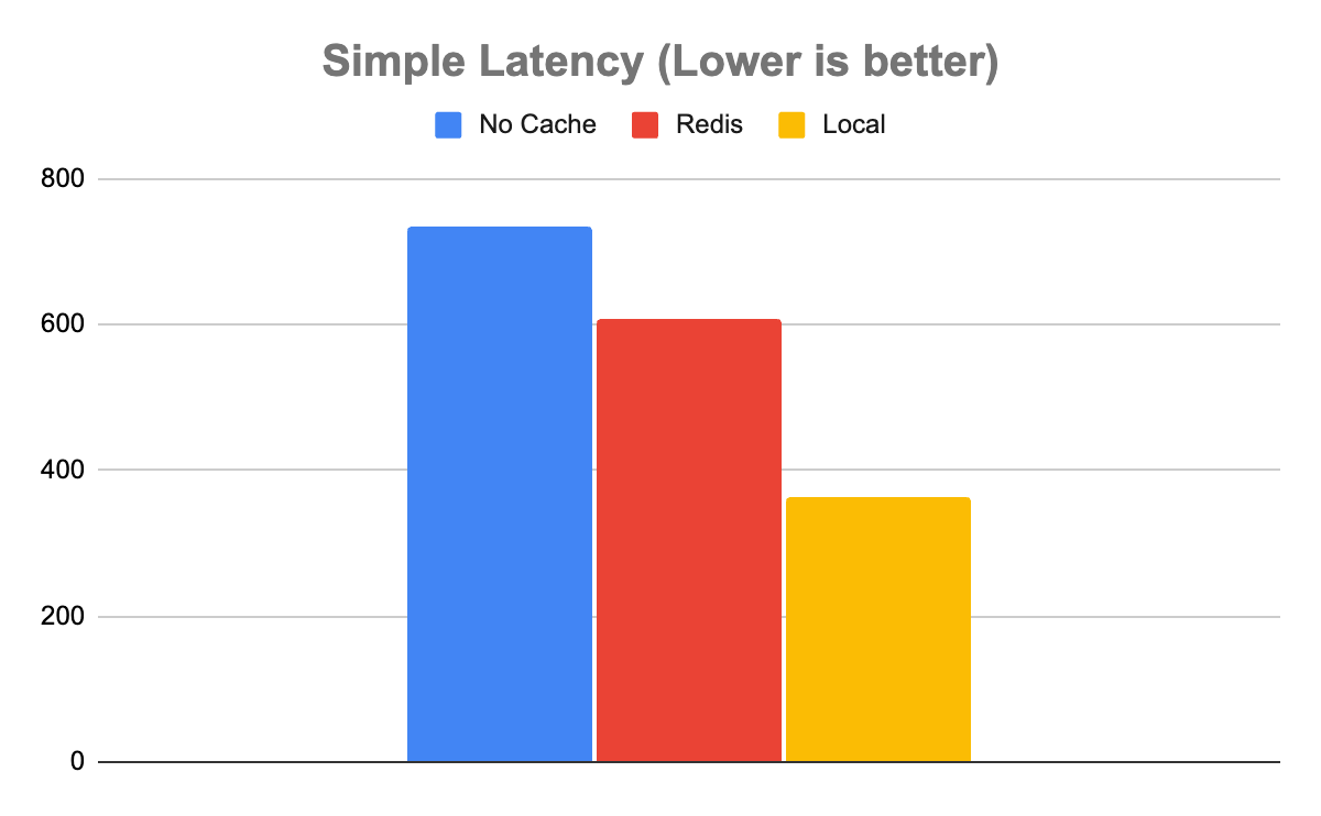
The Simple model tells a slightly more complicated story. In the case of the simple model, not using any cache enabled a throughput of 1,358 inference/sec with a latency of 735 µs. Redis was somewhat faster with a throughput of 1,639 inference/sec and a latency of 608 µs. Local was faster than Redis with a throughput of 2,753 inference/sec with a latency of 363 µs.
This is an important case to note, as not all uses are created equal. The system of record, in this case, may be fast enough and not worth adding the extra system for the 20% boost in throughput of Redis. Even with the halving of latency in the case of the local cache, it may not be worth the resource contention, depending on other factors such as cache hit rate and available system resources.
Best practices for managing trade-offs
As shown in the experiment, the difference between models, expected inputs, and expected outputs is critically important for assessing what, if any, caching is appropriate for your Triton instance.
Whether caching adds value is largely a function of how computationally expensive your queries are. The more computationally expensive your queries, the more each query will benefit from caching.
The relative performance of local versus Redis will largely be a function of how large the output tensors are from the model. The larger the output tensors, the more the transport costs will impact the throughput allowable by Redis.
Of course, the larger the output tensors are, the fewer output tensors you’ll be able to store in the local cache before you run out of room and begin contending with Triton for resources. Fundamentally, these factors need to be balanced when assessing which caching solution works best for your deployment of Triton.
| Benefits | Drawbacks |
| 1. Horizontally scalable 2. Effectively unlimited memory access 3. Enables high availability and disaster recovery 4. Removes resource contention 5. Minimizes cold starts |
A distributed Redis cache requires calls over the network. Naturally, you can expect somewhat lower throughput and higher latency as compared to the local cache. |
Summary
Distributed caching is an old trick that developers use to boost system performance while enabling horizontal scalability and separation of concerns. With the introduction of the Redis Cache for Triton Inference Server, you can now leverage this technique to greatly increase the performance and efficiency of your Triton instance, while managing heavier workloads and enabling multiple Triton instances to share in the same cache. Fundamentally, by offloading caching to Redis, Triton can concentrate its resources on its fundamental role—running inferences.
Get started with Triton Redis Cache and NVIDIA Triton Inference Server. For more information about setting up and administering Redis instances, see redis.io and docs.redis.com.
 Learn to create an end-to-end machine learning pipeline for large datasets with this virtual, hands-on workshop.
 Episode 5 of the NVIDIA CUDA Tutorials Video series is out. Jackson Marusarz, product manager for Compute Developer Tools at NVIDIA, introduces a suite of tools…

 NVIDIA DOCA SDK and acceleration framework empowers developers with extensive libraries, drivers, and APIs to create high-performance applications and services…
 NVIDIA is driving fast-paced innovation in 5G software and hardware across the ecosystem with its OpenRAN-compatible 5G portfolio. Accelerated computing…