From start-ups to large enterprises, businesses use cloud marketplaces to find the new solutions needed to quickly transform their businesses. Cloud…
From start-ups to large enterprises, businesses use cloud marketplaces to find the new solutions needed to quickly transform their businesses. Cloud marketplaces are online storefronts where customers can purchase software and services with flexible billing models, including pay-as-you-go, subscriptions, and privately negotiated offers. Businesses further benefit from committed spending at discount prices and a single source of billing and invoicing that saves time and resources.
NVIDIA Riva state-of-the-art speech and translation AI services are on the largest cloud service providers (CSP) marketplaces:
Companies can quickly find high-performance speech and translation AI that can be fully customized to best fit conversational pipelines such as question and answering services, intelligent virtual assistants, digital avatars, and agent assists for contact centers in different languages.
Organizations can quickly run Riva on the public cloud or integrate it with cloud provider services with greater confidence and a better return on their investment. With NVIDIA Riva in the cloud, you can now get instant access to Riva speech and translation AI through your browser—even if you don’t currently have your own on-premises GPU-accelerated infrastructure.
Purchase NVIDIA Riva from the marketplace, or use existing cloud credits. Contact NVIDIA for discounted private pricing through a Amazon Web Services, Google Cloud Platform, or Microsoft Azure private offer.
In this post and the associated videos, using Spanish-to-English speech-to-speech (S2S) translation as an example, you learn how to prototype and test Riva on a single CSP node. This post also covers deploying Riva in production at scale on a managed Kubernetes cluster.
Prototype and test Riva on a single node
Before launching and scaling a conversational application with Riva, prototype and test on a single node to find defects and improvement areas and ensure perfect production performance.
- Select and launch the Riva virtual machine image (VMI) on the public CSPs
- Access the Riva container on the NVIDIA GPU Cloud (NGC) catalog
- Configure the NGC CLI
- Edit the Riva Skills Quick Start configuration script and deploy the Riva server
- Get started with Riva with tutorial Jupyter notebooks
- Run speech-to-speech (S2S) translation inference
Video 1 explains how to launch a GCP virtual machine instance from the Riva VMI and connect to it from a terminal.
Video 2 shows how to start the Riva Server and run Spanish-to-English speech-to-speech translation in the virtual machine instance.
Select and launch the Riva VMI on a public CSP
The Riva VMI provides a self-contained environment that enables you to run Riva on single nodes in public cloud services. You can quickly launch with the following steps.
Go to your chosen CSP:
Choose the appropriate button to begin configuring the VM instance.
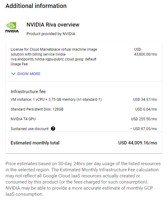
- Set the compute zone, GPU and CPU types, and network security rules. The S2S translation demo should only take 13-14 GB of GPU memory and should be able to run on a 16 GB T4 GPU.
- If necessary, generate an SSH key pair.
Deploy the VM instance and edit it further, if necessary. Connect to the VM instance using SSH and a key file in your local terminal (this is the safest way).
Connecting to a GCP VM instance with SSH and a key file requires the gcloud CLI rather than the built-in SSH tool. Use the following command format:
gcloud compute ssh --project= --zone= -- -L 8888:localhost:8888
If you’ve already added the Project_ID and compute-zone values to your gcloud config, you can omit those flags in the command. The -L flag enables port forwarding, which enables you to launch Jupyter on the VM instance and access it in your local browser as though the Jupyter server were running locally.
Access the Riva container on NGC
The NGC catalog is a curated set of GPU-accelerated AI models and SDKs to help you quickly infuse AI into your applications.
The easiest way to download the Riva containers and desired models into the VM instance is to download the Riva Skills Quick Start resource folder with the appropriate ngc command, edit the provided config.sh script, and run the riva_init.sh and riva_start.sh scripts.
An additional perk for Riva VMI subscribers is access to the NVIDIA AI Enterprise Catalog on NGC.
Configure the NGC CLI to access resources
Your NGC CLI configuration ensures that you can access NVIDIA software resources. The configuration also determines which container registry space you can access.
The Riva VMI already provides the NGC CLI, so you don’t have to download or install it. You do still need to configure it.
Generate an NGC API key, if necessary. At the top right, choose your name and org. Choose Setup, Get API Key, and Generate API Key. Make sure to copy and save your newly generated API key someplace safe.
Run ngc config set and paste in your API key. Set the output format for the results of calls to the NGC CLI and set your org, team, and ACE.
Edit the Riva Skills Quick Start configuration script and deploy the Riva Server
Riva includes Quick Start scripts to help you get started with Riva speech and translation AI services:
- Automatic speech recognition (ASR)
- Text-to-speech (TTS)
- Several natural language processing (NLP) tasks
- Neural machine translation (NMT)
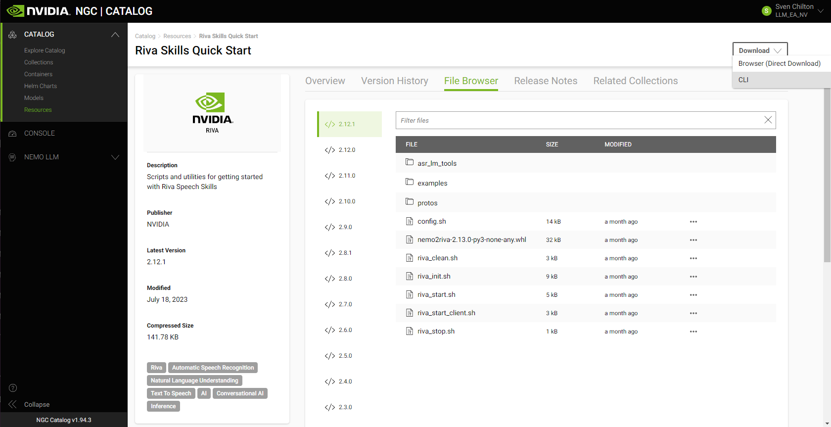
On the asset’s NGC overview page, choose Download. To copy the appropriate NGC CLI command into your VM instance’s terminal, choose CLI:
ngc registry resource download-version "nvidia/riva/riva_quickstart:2.12.1"
At publication time, 2.12.1 is the most recent version of Riva. Check the NGC catalog or the Riva documentation page for the latest version number.
After downloading the Riva Skills Quick Start resource folder in your VM instance’s terminal, implement a Spanish-to-English speech-to-speech (S2S) translation pipeline.
In the Riva Skills Quick Start home directory, edit the config.sh script to tell Riva which services to enable and which model files in the .rmir format to download.
Set service_enabled_nlp=false but leave the other services as true. You need Spanish ASR, Spanish-to-English NMT, and English TTS. There is no need for NLP.
To enable Spanish ASR, change language_code=("en-US") to language_code=("es-US").
Uncomment the line containing rmir_megatronnmt_any_en_500m to enable NMT from Spanish (and any of over 30 additional languages) to English.
To download the desired .rmir files and deploy them, run the following command. riva_init.sh wraps around the riva-deploy command.
bash riva_init.sh config.sh
To start the Riva server, run the following command:
bash riva_start.sh config.sh
If the server doesn’t start, output the relevant Docker logs to a file:
docker logs riva-speech &> docker-logs-riva-speech.txt
Inspect the file. If you see any CUDA out-of-memory errors, your model pipeline is too big for your GPU.
Get started with Riva through Jupyter notebook tutorials
One of the best ways to get started with Riva is to work through the Jupyter notebook tutorials in the /nvidia-riva/tutorials GitHub repo:
git clone https://github.com/nvidia-riva/tutorials.git
The VMI already contains a miniconda Python distribution, which includes Jupyter. Create a new conda environment from the base (default) environment in which to install dependencies, then launch Jupyter.
Clone the base (default) environment:
conda create --name conda-riva-tutorials --clone base
Activate the new environment:
conda activate conda-riva-tutorials
Install an iPython kernel for the new environment:
ipython kernel install --user --name=conda-riva-tutorials
Launch Jupyter Lab:
jupyter lab --allow-root --ip 0.0.0.0 --port 8888
If you set up port forwarding when connecting to the VM instance with gcloud compute ssh, choose the link containing 127.0.0.1 to run Jupyter Lab in your local browser. If not, enter the following into your browser bar to run Jupyter Lab:
- Your VM instance’s external IP address
- A colon (:)
- The port number (presumably
8888) /lab?token=
If you don’t want to copy and paste the token in the browser bar, the browser asks you to enter the token in a dialog box instead.
Run the speech-to-speech translation demo
This speech-to-speech (S2S) demonstration consists of a modified version of the nmt-python-basics.ipynb tutorial notebook. To carry it out, perform the following steps.
Import the necessary modules:
import IPython.display as ipd

import numpy as np

import riva.client
Create a Riva client and connect to the Riva server:
auth = riva.client.Auth(uri="localhost:50051")
riva_nmt_client = riva.client.NeuralMachineTranslationClient(auth)
Load the audio file:
my_wav_file = "ASR-Demo-2-Spanish-Non-Native-Elena.wav"
The audio file contains a clip of a colleague reading a line from Miguel de Cervantes’ celebrated novel Don Quixote, “Cuando la vida misma parece lunática, ¿quién sabe dónde está la locura?”
This can be translated into English as, “When life itself seems lunatic, who knows where madness lies?”
Set up an audio chunk iterator, that is, divide the audio file into chunks no larger than a given number of frames:
audio_chunk_iterator = riva.client.AudioChunkFileIterator(my_wav_file, chunk_n_frames=4800)
Define an S2S config, composed of a sequence of ASR, NMT, and TTS configs:
s2s_config = riva.client.StreamingTranslateSpeechToSpeechConfig(
          asr_config = riva.client.StreamingRecognitionConfig(
              config=riva.client.RecognitionConfig(
                  encoding=riva.client.AudioEncoding.LINEAR_PCM,
                  language_code='es-US',    # Spanish ASR model
                  max_alternatives=1,
                  profanity_filter=False,
                  enable_automatic_punctuation=True,
                  verbatim_transcripts=not True,
                  sample_rate_hertz=16000,
                  audio_channel_count=1,
              ),
              interim_results=True,
          ),
          translation_config = riva.client.TranslationConfig(
              source_language_code="es-US",    # Source language is Spanish
              target_language_code='en-US',    # Target language is English
              model_name='megatronnmt_any_en_500m',
          ),
          tts_config = riva.client.SynthesizeSpeechConfig(
              encoding=1,
              sample_rate_hz=44100,
              voice_name="English-US.Female-1", # Default EN female voice
              language_code="en-US",
          ),
      )
Make gRPC requests to the Riva Speech API server:
responses = riva_nmt_client.streaming_s2s_response_generator(
          audio_chunks=audio_chunk_iterator,
          streaming_config=s2s_config)
Listen to the streaming response:
# Create an empty array to store the receiving audio buffer
empty = np.array([])
# Send requests and listen to streaming response from the S2S service
for i, rep in enumerate(responses):
    audio_samples = np.frombuffer(rep.speech.audio, dtype=np.int16) / (2**15)
    print("Chunk: ",i)
    try:
        ipd.display(ipd.Audio(audio_samples, rate=44100))
    except:
        print("Empty response")
    empty = np.concatenate((empty, audio_samples))
# Full translated synthesized speech
print("Final synthesis:")
ipd.display(ipd.Audio(empty, rate=44100))
This yields clips of synthesized speech in chunks and a final, fully assembled clip. The synthesized voice in the final clip should say, “When life itself seems lunatic, who knows where madness lies?”
Deploy Riva on a managed Kubernetes platform
After launching a Riva VMI and gaining access to the enterprise catalog, you can also deploy Riva to the various supported managed Kubernetes platforms like AKS, Amazon EKS, and GKE. These managed Kubernetes platforms are ideal for production-grade deployments because they enable seamless automated deployment, easy scalability, and efficient operability.
To help you get started, this post guides you through an example deployment for Riva on a GKE cluster. By combining the power of Terraform and Helm, you can quickly stand up production-grade deployments.
- Set up a Kubernetes cluster on a managed Kubernetes platform with the NVIDIA Terraform modules
- Deploy the Riva server on the Kubernetes cluster with a Helm chart
- Interact with Riva on the Kubernetes cluster
Video 3 explains how to set up and run Riva on Google Kubernetes Engine (GKE) with Terraform.
Video 4 shows how to scale up and out speech AI inference by deploying Riva on the Kubernetes cluster with Helm.
Set up the GKE cluster with the NVIDIA Terraform modules
The NVIDIA Terraform modules make it easy to deploy a Riva-ready GKE cluster. For more information, see the /nvidia-terraform-modules GitHub repo.
To get started, clone the repo and install the prerequisites on a machine:
- kubectl
- gcloud CLI
- Make sure that you also install the GKE authentication plugin by running
gcloud components install gke-gcloud-auth-plugin
- Make sure that you also install the GKE authentication plugin by running
- GCP account where you have Kubernetes Engine Admin permissions
- Terraform (CLI)
From within the nvidia-terraform-modules/gke directory, ensure that you have active credentials set with the gcloud CLI.
Update terraform.tfvars by uncommenting cluster_name and region and filling out the values specific to your project. By default, this module deploys the cluster into a new VPC. To deploy the cluster into an existing VPC, you must also uncomment and set the existing_vpc_details variable.
Alternatively, you can change any variable names or parameters in any of the following ways:
- Add them directly to
variables.tf. - Pass them in from the command line with the
-varflag. - Pass them in as environment variables.
- Pass them in from the command line when prompted.
In variables.tf, update the following variables for use by Riva: GPU type and region.
Select a supported GPU type:
variable "gpu_type" {
  default     = "nvidia-tesla-t4"
  description = "GPU SKU To attach to Holoscan GPU Node (eg. nvidia-tesla-k80)"
}
(Optional) Select your region:
variable "region" {
  default     = "us-west1"
  description = "The Region resources (VPC, GKE, Compute Nodes) will be created in"
}
Run gcloud auth application-default login to make your Google credentials available to the terraform executable. For more information, see Assigning values to root module variables in the Terraform documentation.
terraform init: Initialize the configuration.terraform plan: See what will be applied.terraform apply: Apply the code against your GKE environment.
Connect to the cluster with kubectl by running the following command after the cluster is created:
gcloud container clusters get-credentials --region=
To delete cloud infrastructure provisioned by Terraform, run terraform destroy.
The NVIDIA Terraform modules can also be used for deployments in other CSPs and follow a similar pattern. For more information about deploying AKS and EKS clusters, see the /nvidia-terraform-modules GitHub repo.
Deploy the Riva Speech Skills API with a Helm chart
The Riva speech skills Helm chart is designed to automate deployment to a Kubernetes cluster. After downloading the Helm chart, minor adjustments adapt the chart to the way Riva is used in the rest of this post.
Start by downloading and untarring the Riva API Helm chart. The 2.12.1 version is the most recent as of this post. To download a different version of the Helm chart, replace VERSION_TAG with the specific version needed in the following code example:
export NGC_CLI_API_KEY=
export VERSION_TAG="2.12.1"
helm fetch https://helm.ngc.nvidia.com/nvidia/riva/charts/riva-api-${VERSION_TAG}.tgz --username='$oauthtoken' --password=$NGC_CLI_API_KEY
tar -xvzf riva-api-${VERSION_TAG}.tgz
In the riva-api folder, modify the following files as noted.
In the values.yaml file, in modelRepoGenerator.ngcModelConfigs.tritonGroup0, comment or uncomment specific models or change language codes as needed.
For the S2S pipeline used earlier:
- Change the language code in the ASR model from US English to Latin American Spanish, so that
rmir_asr_conformer_en_us_str_thrbecomesrmir_asr_conformer_es_us_str_thr. - Uncomment the line containing
rmir_megatronnmt_any_en_500m. - Ensure that
service.typeis set toClusterIPrather thanLoadBalancer. This exposes the service only to other services within the cluster, such as the proxy service installed later in this post.
In the templates/deployment.yaml file, follow up by adding a node selector constraint to ensure that Riva is only deployed on the correct GPU resources. Attach it to a node pool (called a node group in Amazon EKS). You can get this from the GCP console or by running the appropriate gcloud commands in your terminal:
$ gcloud container clusters list
NAME                         LOCATION  MASTER_VERSION  MASTER_IP       MACHINE_TYPE   NODE_VERSION    NUM_NODES  STATUS
riva-in-the-cloud-blog-demo  us-west1  1.27.3-gke.100  35.247.68.177   n1-standard-4  1.27.3-gke.100  3          RUNNING

$ gcloud container node-pools list --cluster=riva-in-the-cloud-blog-demo --location=us-west1
NAME                                     MACHINE_TYPE   DISK_SIZE_GB  NODE_VERSION
tf-riva-in-the-cloud-blog-demo-cpu-pool  n1-standard-4  100           1.27.3-gke.100
tf-riva-in-the-cloud-blog-demo-gpu-pool  n1-standard-4  100           1.27.3-gke.100
In spec.template.spec, add the following with your node pool name from earlier:
nodeSelector:
  cloud.google.com/gke-nodepool: tf-riva-in-the-cloud-blog-demo-gpu-pool
Ensure that you are in a working directory with /riva-api as a subdirectory, then install the Riva Helm chart. You can explicitly override variables from the values.yaml file.
helm install riva-api riva-api/
    --set ngcCredentials.password=`echo -n $NGC_CLI_API_KEY | base64 -w0`
    --set modelRepoGenerator.modelDeployKey=`echo -n tlt_encode | base64 -w0`
The Helm chart runs two containers in order:
- A
riva-model-initcontainer that downloads and deploys the models. - A
riva-speech-apicontainer to start the speech service API.
Depending on the number of models, the initial model deployment could take an hour or more. To monitor the deployment, use kubectl to describe the riva-api Pod and to watch the container logs.
export pod=`kubectl get pods | cut -d " " -f 1 | grep riva-api`
kubectl describe pod $pod
kubectl logs -f $pod -c riva-model-init
kubectl logs -f $pod -c riva-speech-api
The Riva server is now deployed.
Interact with Riva on the GKE cluster
While this method of interacting with the server is probably not ideally suited to production environments, you can run the S2S translation demo from anywhere outside the GKE cluster by changing the URI in the call to riva.client.Auth so that the Riva Python client sends inference requests to the riva-api service on the GKE cluster rather than the local host. Obtain the appropriate URI with kubectl:
$ kubectl get services
NAME         TYPE           CLUSTER-IP       EXTERNAL-IP    PORT(S)                                                        AGE
kubernetes   ClusterIP      10.155.240.1              443/TCP                                                        1h
riva-api     LoadBalancer   10.155.243.119   34.127.90.22   8000:30623/TCP,8001:30542/TCP,8002:32113/TCP,50051:30842/TCP   1h
No port forwarding is taking place here. To run the Spanish-to-English S2S translation pipeline on the GKE cluster from a Jupyter notebook outside the cluster, change the following line:
auth = riva.client.Auth(uri="localhost:50051")
Here’s the desired line:
auth = riva.client.Auth(uri=":50051")
There are multiple ways to interact with the server. One method involves deploying IngressRoute through a Traefik Edge router deployable through Helm. For more information, see Deploying the Traefik edge router.
NVIDIA also provides an opinionated production deployment recipe through the Speech AI Workflows, Audio Transcription, Intelligent Virtual Assistant. For more information, see the Technical Brief.
Summary
NVIDIA Riva is available on the Amazon Web Services, Google Cloud, and Microsoft Azure marketplaces. Get started with prototyping and testing Riva in the cloud on a single node through quickly deployable VMIs. For more information, see the NVIDIA Riva on GCP videos.
Production-grade Riva deployments on Managed Kubernetes are easy with NVIDIA Terraform modules. For more information, see the NVIDIA Riva on GKE videos.
Deploy Riva on CSP compute resources with cloud credits by purchasing a license from a CSP marketplace:
You can also reach out to NVIDIA through the Amazon Web Services, Google Cloud, or Microsoft Azure forms for discount pricing with private offers.
 Generative AI has become a transformative force of our era, empowering organizations spanning every industry to achieve unparalleled levels of productivity,…


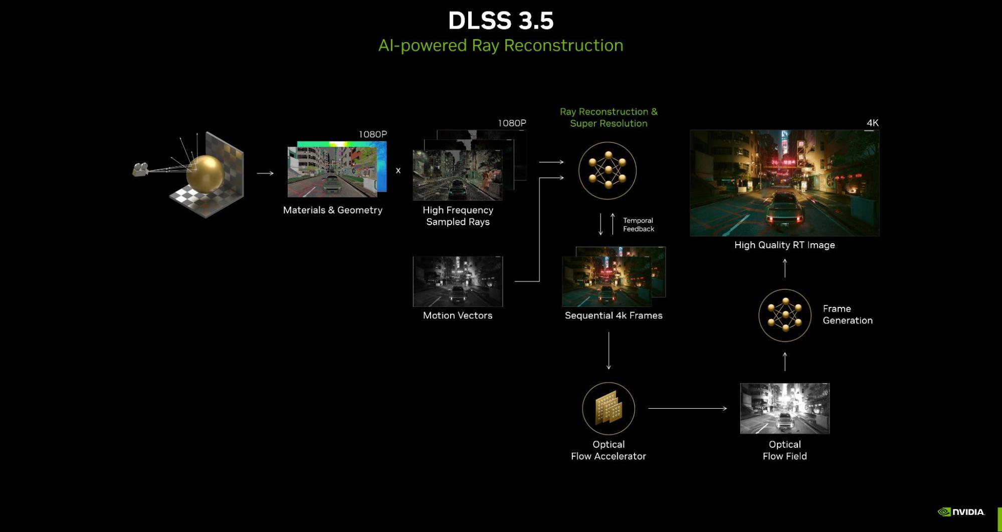
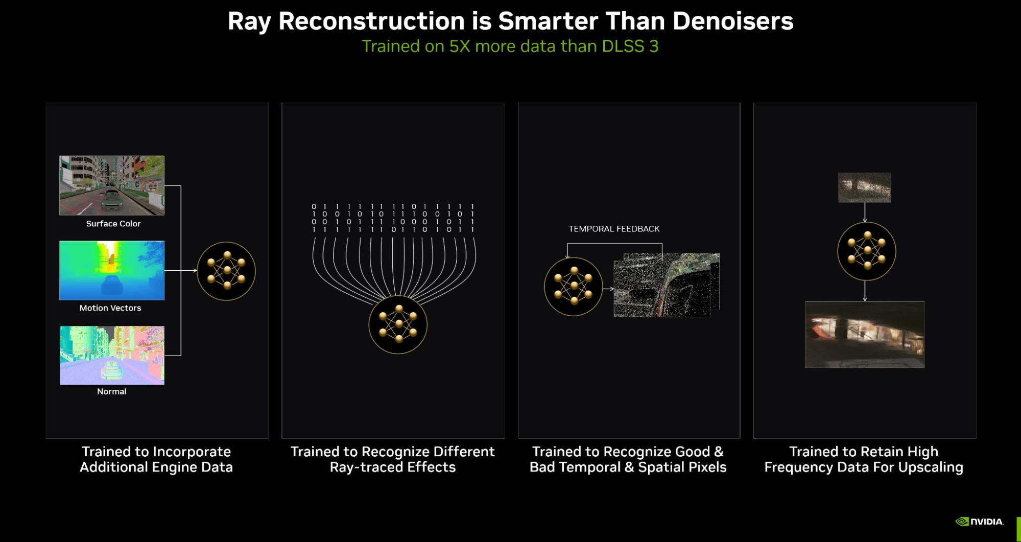
 Since 2018, NVIDIA DLSS has leveraged AI to enable gamers and creators to increase performance and crank up their quality. Over time, this solution has evolved…