
The latest advancements in AI for gaming are in the spotlight today at Gamescom, the world’s largest gaming conference, as NVIDIA introduced a host of technologies, starting with DLSS 3.5, the next step forward of its breakthrough AI neural rendering technology. DLSS 3.5, NVIDIA’s latest innovation in AI-powered graphics is an image quality upgrade incorporated Read article >
On the eve of Gamescom, NVIDIA announced NVIDIA DLSS 3.5 featuring Ray Reconstruction — a new neural rendering AI model that creates more beautiful and realistic ray-traced visuals than traditional rendering methods — for real-time 3D creative apps and games.
Bill Dally — one of the world’s foremost computer scientists and head of NVIDIA’s research efforts — will describe the forces driving accelerated computing and AI in his keynote address at Hot Chips, an annual gathering of leading processor and system architects. Dally will detail advances in GPU silicon, systems and software that are delivering Read article >
Bill Dally — one of the world’s foremost computer scientists and head of NVIDIA’s research efforts — will describe the forces driving accelerated computing and AI in his keynote address at Hot Chips, an annual gathering of leading processor and system architects. Dally will detail advances in GPU silicon, systems and software that are delivering Read article >
Categories
Event: Speech AI Day
 On Sept. 20, join experts from leading companies at NVIDIA-hosted Speech AI Day.
On Sept. 20, join experts from leading companies at NVIDIA-hosted Speech AI Day.
Categories
Google at Interspeech 2023

This week, the 24th Annual Conference of the International Speech Communication Association (INTERSPEECH 2023) is being held in Dublin, Ireland, representing one of the world’s most extensive conferences on research and technology of spoken language understanding and processing. Experts in speech-related research fields gather to take part in oral presentations and poster sessions and to build collaborations across the globe.
We are excited to be a Platinum Sponsor of INTERSPEECH 2023, where we will be showcasing more than 20 research publications and supporting a number of workshops and special sessions. We welcome in-person attendees to drop by the Google Research booth to meet our researchers and participate in Q&As and demonstrations of some of our latest speech technologies, which help to improve accessibility and provide convenience in communication for billions of users. In addition, online attendees are encouraged to visit our virtual booth in Topia where you can get up-to-date information on research and opportunities at Google. Visit the @GoogleAI Twitter account to find out about Google booth activities (e.g., demos and Q&A sessions). You can also learn more about the Google research being presented at INTERSPEECH 2023 below (Google affiliations in bold).
Board and Organizing Committee
ISCA Board, Technical Committee Chair: Bhuvana Ramabhadran
Area Chairs include:
Analysis of Speech and Audio Signals: Richard Rose
Speech Synthesis and Spoken Language Generation: Rob Clark
Special Areas: Tara Sainath
Satellite events
VoxCeleb Speaker Recognition Challenge 2023 (VoxSRC-23)
Organizers include: Arsha Nagrani
ISCA Speech Synthesis Workshop (SSW12)
Speakers include: Rob Clark
Keynote talk – ISCA Medalist
Bridging Speech Science and Technology — Now and Into the Future
Speaker: Shrikanth Narayanan
Survey Talk
Speech Compression in the AI Era
Speaker: Jan Skoglund
Special session papers
Cascaded Encoders for Fine-Tuning ASR Models on Overlapped Speech
Richard Rose, Oscar Chang, Olivier Siohan
TokenSplit: Using Discrete Speech Representations for Direct, Refined, and Transcript-Conditioned Speech Separation and Recognition
Hakan Erdogan, Scott Wisdom, Xuankai Chang*, Zalán Borsos, Marco Tagliasacchi, Neil Zeghidour, John R. Hershey
Papers
DeePMOS: Deep Posterior Mean-Opinion-Score of Speech
Xinyu Liang, Fredrik Cumlin, Christian Schüldt, Saikat Chatterjee
O-1: Self-Training with Oracle and 1-Best Hypothesis
Murali Karthick Baskar, Andrew Rosenberg, Bhuvana Ramabhadran, Kartik Audhkhasi
Re-investigating the Efficient Transfer Learning of Speech Foundation Model Using Feature Fusion Methods
Zhouyuan Huo, Khe Chai Sim, Dongseong Hwang, Tsendsuren Munkhdalai, Tara N. Sainath, Pedro Moreno
MOS vs. AB: Evaluating Text-to-Speech Systems Reliably Using Clustered Standard Errors
Joshua Camp, Tom Kenter, Lev Finkelstein, Rob Clark
LanSER: Language-Model Supported Speech Emotion Recognition
Taesik Gong, Josh Belanich, Krishna Somandepalli, Arsha Nagrani, Brian Eoff, Brendan Jou
Modular Domain Adaptation for Conformer-Based Streaming ASR
Qiujia Li, Bo Li, Dongseong Hwang, Tara N. Sainath, Pedro M. Mengibar
On Training a Neural Residual Acoustic Echo Suppressor for Improved ASR
Sankaran Panchapagesan, Turaj Zakizadeh Shabestary, Arun Narayanan
MD3: The Multi-dialect Dataset of Dialogues
Jacob Eisenstein, Vinodkumar Prabhakaran, Clara Rivera, Dorottya Demszky, Devyani Sharma
Dual-Mode NAM: Effective Top-K Context Injection for End-to-End ASR
Zelin Wu, Tsendsuren Munkhdalai, Pat Rondon, Golan Pundak, Khe Chai Sim, Christopher Li
Using Text Injection to Improve Recognition of Personal Identifiers in Speech
Yochai Blau, Rohan Agrawal, Lior Madmony, Gary Wang, Andrew Rosenberg, Zhehuai Chen, Zorik Gekhman, Genady Beryozkin, Parisa Haghani, Bhuvana Ramabhadran
How to Estimate Model Transferability of Pre-trained Speech Models?
Zih-Ching Chen, Chao-Han Huck Yang*, Bo Li, Yu Zhang, Nanxin Chen, Shuo-yiin Chang, Rohit Prabhavalkar, Hung-yi Lee, Tara N. Sainath
Improving Joint Speech-Text Representations Without Alignment
Cal Peyser, Zhong Meng, Ke Hu, Rohit Prabhavalkar, Andrew Rosenberg, Tara N. Sainath, Michael Picheny, Kyunghyun Cho
Text Injection for Capitalization and Turn-Taking Prediction in Speech Models
Shaan Bijwadia, Shuo-yiin Chang, Weiran Wang, Zhong Meng, Hao Zhang, Tara N. Sainath
Streaming Parrotron for On-Device Speech-to-Speech Conversion
Oleg Rybakov, Fadi Biadsy, Xia Zhang, Liyang Jiang, Phoenix Meadowlark, Shivani Agrawal
Semantic Segmentation with Bidirectional Language Models Improves Long-Form ASR
W. Ronny Huang, Hao Zhang, Shankar Kumar, Shuo-yiin Chang, Tara N. Sainath
Universal Automatic Phonetic Transcription into the International Phonetic Alphabet
Chihiro Taguchi, Yusuke Sakai, Parisa Haghani, David Chiang
Mixture-of-Expert Conformer for Streaming Multilingual ASR
Ke Hu, Bo Li, Tara N. Sainath, Yu Zhang, Francoise Beaufays
Real Time Spectrogram Inversion on Mobile Phone
Oleg Rybakov, Marco Tagliasacchi, Yunpeng Li, Liyang Jiang, Xia Zhang, Fadi Biadsy
2-Bit Conformer Quantization for Automatic Speech Recognition
Oleg Rybakov, Phoenix Meadowlark, Shaojin Ding, David Qiu, Jian Li, David Rim, Yanzhang He
LibriTTS-R: A Restored Multi-speaker Text-to-Speech Corpus
Yuma Koizumi, Heiga Zen, Shigeki Karita, Yifan Ding, Kohei Yatabe, Nobuyuki Morioka, Michiel Bacchiani, Yu Zhang, Wei Han, Ankur Bapna
PronScribe: Highly Accurate Multimodal Phonemic Transcription from Speech and Text
Yang Yu, Matthew Perez*, Ankur Bapna, Fadi Haik, Siamak Tazari, Yu Zhang
Label Aware Speech Representation Learning for Language Identification
Shikhar Vashishth, Shikhar Bharadwaj, Sriram Ganapathy, Ankur Bapna, Min Ma, Wei Han, Vera Axelrod, Partha Talukdar
* Work done while at Google
The verdict is in: A GeForce NOW Ultimate membership raises the bar on gaming. Members have been tackling the Ultimate KovvaK’s challenge head-on and seeing for themselves how the power of Ultimate improves their gaming with 240 frames per second streaming. The popular training title that helps gamers improve their aim fully launches in the Read article >
Categories
Wanna help judge SoME3?
There has been great progress towards adapting large language models (LLMs) to accommodate multimodal inputs for tasks including image captioning, visual question answering (VQA), and open vocabulary recognition. Despite such achievements, current state-of-the-art visual language models (VLMs) perform inadequately on visual information seeking datasets, such as Infoseek and OK-VQA, where external knowledge is required to answer the questions.
 |
| Examples of visual information seeking queries where external knowledge is required to answer the question. Images are taken from the OK-VQA dataset. |
In “AVIS: Autonomous Visual Information Seeking with Large Language Models”, we introduce a novel method that achieves state-of-the-art results on visual information seeking tasks. Our method integrates LLMs with three types of tools: (i) computer vision tools for extracting visual information from images, (ii) a web search tool for retrieving open world knowledge and facts, and (iii) an image search tool to glean relevant information from metadata associated with visually similar images. AVIS employs an LLM-powered planner to choose tools and queries at each step. It also uses an LLM-powered reasoner to analyze tool outputs and extract key information. A working memory component retains information throughout the process.
 |
| An example of AVIS’s generated workflow for answering a challenging visual information seeking question. The input image is taken from the Infoseek dataset. |
Comparison to previous work
Recent studies (e.g., Chameleon, ViperGPT and MM-ReAct) explored adding tools to LLMs for multimodal inputs. These systems follow a two-stage process: planning (breaking down questions into structured programs or instructions) and execution (using tools to gather information). Despite success in basic tasks, this approach often falters in complex real-world scenarios.
There has also been a surge of interest in applying LLMs as autonomous agents (e.g., WebGPT and ReAct). These agents interact with their environment, adapt based on real-time feedback, and achieve goals. However, these methods do not restrict the tools that can be invoked at each stage, leading to an immense search space. Consequently, even the most advanced LLMs today can fall into infinite loops or propagate errors. AVIS tackles this via guided LLM use, influenced by human decisions from a user study.
Informing LLM decision making with a user study
Many of the visual questions in datasets such as Infoseek and OK-VQA pose a challenge even for humans, often requiring the assistance of various tools and APIs. An example question from the OK-VQA dataset is shown below. We conducted a user study to understand human decision-making when using external tools.
 |
| We conducted a user study to understand human decision-making when using external tools. Image is taken from the OK-VQA dataset. |
The users were equipped with an identical set of tools as our method, including PALI, PaLM, and web search. They received input images, questions, detected object crops, and buttons linked to image search results. These buttons offered diverse information about the detected object crops, such as knowledge graph entities, similar image captions, related product titles, and identical image captions.
We record user actions and outputs and use it as a guide for our system in two key ways. First, we construct a transition graph (shown below) by analyzing the sequence of decisions made by users. This graph defines distinct states and restricts the available set of actions at each state. For example, at the start state, the system can take only one of these three actions: PALI caption, PALI VQA, or object detection. Second, we use the examples of human decision-making to guide our planner and reasoner with relevant contextual instances to enhance the performance and effectiveness of our system.
 |
| AVIS transition graph. |
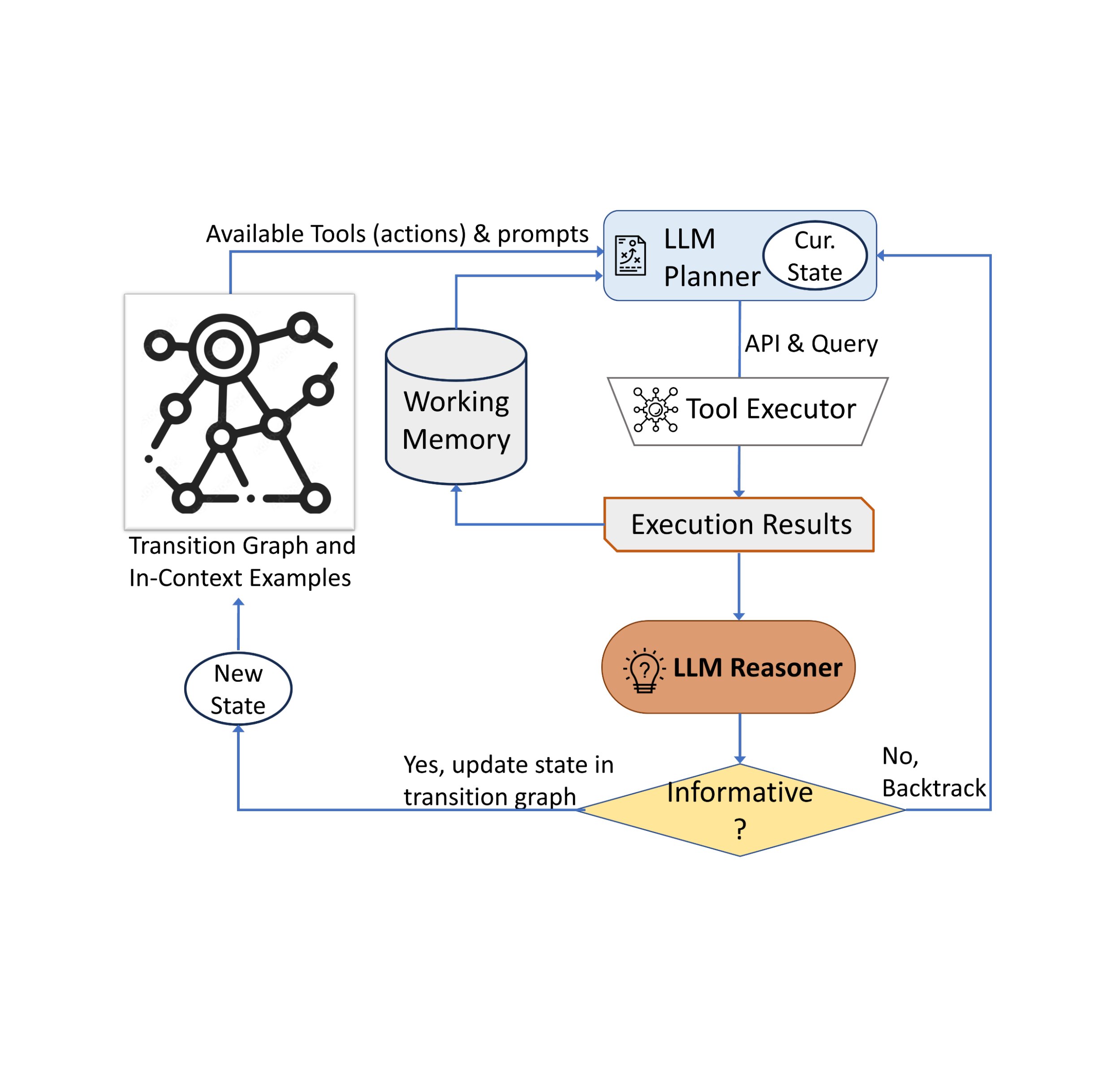
General framework
Our approach employs a dynamic decision-making strategy designed to respond to visual information-seeking queries. Our system has three primary components. First, we have a planner to determine the subsequent action, including the appropriate API call and the query it needs to process. Second, we have a working memory that retains information about the results obtained from API executions. Last, we have a reasoner, whose role is to process the outputs from the API calls. It determines whether the obtained information is sufficient to produce the final response, or if additional data retrieval is required.
The planner undertakes a series of steps each time a decision is required regarding which tool to employ and what query to send to it. Based on the present state, the planner provides a range of potential subsequent actions. The potential action space may be so large that it makes the search space intractable. To address this issue, the planner refers to the transition graph to eliminate irrelevant actions. The planner also excludes the actions that have already been taken before and are stored in the working memory.
Next, the planner collects a set of relevant in-context examples that are assembled from the decisions previously made by humans during the user study. With these examples and the working memory that holds data collected from past tool interactions, the planner formulates a prompt. The prompt is then sent to the LLM, which returns a structured answer, determining the next tool to be activated and the query to be dispatched to it. This design allows the planner to be invoked multiple times throughout the process, thereby facilitating dynamic decision-making that gradually leads to answering the input query.
We employ a reasoner to analyze the output of the tool execution, extract the useful information and decide into which category the tool output falls: informative, uninformative, or final answer. Our method utilizes the LLM with appropriate prompting and in-context examples to perform the reasoning. If the reasoner concludes that it’s ready to provide an answer, it will output the final response, thus concluding the task. If it determines that the tool output is uninformative, it will revert back to the planner to select another action based on the current state. If it finds the tool output to be useful, it will modify the state and transfer control back to the planner to make a new decision at the new state.
 |
| AVIS employs a dynamic decision-making strategy to respond to visual information-seeking queries. |
Results
We evaluate AVIS on Infoseek and OK-VQA datasets. As shown below, even robust visual-language models, such as OFA and PaLI, fail to yield high accuracy when fine-tuned on Infoseek. Our approach (AVIS), without fine-tuning, achieves 50.7% accuracy on the unseen entity split of this dataset.
 |
| AVIS visual question answering results on Infoseek dataset. AVIS achieves higher accuracy in comparison to previous baselines based on PaLI, PaLM and OFA. |
Our results on the OK-VQA dataset are shown below. AVIS with few-shot in-context examples achieves an accuracy of 60.2%, higher than most of the previous works. AVIS achieves lower but comparable accuracy in comparison to the PALI model fine-tuned on OK-VQA. This difference, compared to Infoseek where AVIS outperforms fine-tuned PALI, is due to the fact that most question-answer examples in OK-VQA rely on common sense knowledge rather than on fine-grained knowledge. Therefore, PaLI is able to encode such generic knowledge in the model parameters and doesn’t require external knowledge.
 |
| Visual question answering results on A-OKVQA. AVIS achieves higher accuracy in comparison to previous works that use few-shot or zero-shot learning, including Flamingo, PaLI and ViperGPT. AVIS also achieves higher accuracy than most of the previous works that are fine-tuned on OK-VQA dataset, including REVEAL, ReVIVE, KAT and KRISP, and achieves results that are close to the fine-tuned PaLI model. |
Conclusion
We present a novel approach that equips LLMs with the ability to use a variety of tools for answering knowledge-intensive visual questions. Our methodology, anchored in human decision-making data collected from a user study, employs a structured framework that uses an LLM-powered planner to dynamically decide on tool selection and query formation. An LLM-powered reasoner is tasked with processing and extracting key information from the output of the selected tool. Our method iteratively employs the planner and reasoner to leverage different tools until all necessary information required to answer the visual question is amassed.
Acknowledgements
This research was conducted by Ziniu Hu, Ahmet Iscen, Chen Sun, Kai-Wei Chang, Yizhou Sun, David A. Ross, Cordelia Schmid and Alireza Fathi.
Categories
Take a Free NVIDIA Technical Training Course
 Join the free NVIDIA Developer Program and enroll in a course from the NVIDIA Deep Learning Institute.
Join the free NVIDIA Developer Program and enroll in a course from the NVIDIA Deep Learning Institute.