Modern neural networks have achieved impressive performance across a variety of applications, such as language, mathematical reasoning, and vision. However, these networks often use large architectures that require lots of computational resources. This can make it impractical to serve such models to users, especially in resource-constrained environments like wearables and smartphones. A widely used approach to mitigate the inference costs of pre-trained networks is to prune them by removing some of their weights, in a way that doesn’t significantly affect utility. In standard neural networks, each weight defines a connection between two neurons. So after weights are pruned, the input will propagate through a smaller set of connections and thus requires less computational resources.
 |
| Original network vs. a pruned network. |
Pruning methods can be applied at different stages of the network’s training process: post, during, or before training (i.e., immediately after weight initialization). In this post, we focus on the post-training setting: given a pre-trained network, how can we determine which weights should be pruned? One popular method is magnitude pruning, which removes weights with the smallest magnitude. While efficient, this method doesn’t directly consider the effect of removing weights on the network’s performance. Another popular paradigm is optimization-based pruning, which removes weights based on how much their removal impacts the loss function. Although conceptually appealing, most existing optimization-based approaches seem to face a serious tradeoff between performance and computational requirements. Methods that make crude approximations (e.g., assuming a diagonal Hessian matrix) can scale well, but have relatively low performance. On the other hand, while methods that make fewer approximations tend to perform better, they appear to be much less scalable.
In “Fast as CHITA: Neural Network Pruning with Combinatorial Optimization”, presented at ICML 2023, we describe how we developed an optimization-based approach for pruning pre-trained neural networks at scale. CHITA (which stands for “Combinatorial Hessian-free Iterative Thresholding Algorithm”) outperforms existing pruning methods in terms of scalability and performance tradeoffs, and it does so by leveraging advances from several fields, including high-dimensional statistics, combinatorial optimization, and neural network pruning. For example, CHITA can be 20x to 1000x faster than state-of-the-art methods for pruning ResNet and improves accuracy by over 10% in many settings.
Overview of contributions
CHITA has two notable technical improvements over popular methods:
- Efficient use of second-order information: Pruning methods that use second-order information (i.e., relating to second derivatives) achieve the state of the art in many settings. In the literature, this information is typically used by computing the Hessian matrix or its inverse, an operation that is very difficult to scale because the Hessian size is quadratic with respect to the number of weights. Through careful reformulation, CHITA uses second-order information without having to compute or store the Hessian matrix explicitly, thus allowing for more scalability.
- Combinatorial optimization: Popular optimization-based methods use a simple optimization technique that prunes weights in isolation, i.e., when deciding to prune a certain weight they don’t take into account whether other weights have been pruned. This could lead to pruning important weights because weights deemed unimportant in isolation may become important when other weights are pruned. CHITA avoids this issue by using a more advanced, combinatorial optimization algorithm that takes into account how pruning one weight impacts others.
In the sections below, we discuss CHITA’s pruning formulation and algorithms.
A computation-friendly pruning formulation
There are many possible pruning candidates, which are obtained by retaining only a subset of the weights from the original network. Let k be a user-specified parameter that denotes the number of weights to retain. Pruning can be naturally formulated as a best-subset selection (BSS) problem: among all possible pruning candidates (i.e., subsets of weights) with only k weights retained, the candidate that has the smallest loss is selected.
 |
| Pruning as a BSS problem: among all possible pruning candidates with the same total number of weights, the best candidate is defined as the one with the least loss. This illustration shows four candidates, but this number is generally much larger. |
Solving the pruning BSS problem on the original loss function is generally computationally intractable. Thus, similar to previous work, such as OBD and OBS, we approximate the loss with a quadratic function by using a second-order Taylor series, where the Hessian is estimated with the empirical Fisher information matrix. While gradients can be typically computed efficiently, computing and storing the Hessian matrix is prohibitively expensive due to its sheer size. In the literature, it is common to deal with this challenge by making restrictive assumptions on the Hessian (e.g., diagonal matrix) and also on the algorithm (e.g., pruning weights in isolation).
CHITA uses an efficient reformulation of the pruning problem (BSS using the quadratic loss) that avoids explicitly computing the Hessian matrix, while still using all the information from this matrix. This is made possible by exploiting the low-rank structure of the empirical Fisher information matrix. This reformulation can be viewed as a sparse linear regression problem, where each regression coefficient corresponds to a certain weight in the neural network. After obtaining a solution to this regression problem, coefficients set to zero will correspond to weights that should be pruned. Our regression data matrix is (n x p), where n is the batch (sub-sample) size and p is the number of weights in the original network. Typically n << p, so storing and operating with this data matrix is much more scalable than common pruning approaches that operate with the (p x p) Hessian.
 |
| CHITA reformulates the quadratic loss approximation, which requires an expensive Hessian matrix, as a linear regression (LR) problem. The LR’s data matrix is linear in p, which makes the reformulation more scalable than the original quadratic approximation. |
Scalable optimization algorithms
CHITA reduces pruning to a linear regression problem under the following sparsity constraint: at most k regression coefficients can be nonzero. To obtain a solution to this problem, we consider a modification of the well-known iterative hard thresholding (IHT) algorithm. IHT performs gradient descent where after each update the following post-processing step is performed: all regression coefficients outside the Top-k (i.e., the k coefficients with the largest magnitude) are set to zero. IHT typically delivers a good solution to the problem, and it does so iteratively exploring different pruning candidates and jointly optimizing over the weights.
Due to the scale of the problem, standard IHT with constant learning rate can suffer from very slow convergence. For faster convergence, we developed a new line-search method that exploits the problem structure to find a suitable learning rate, i.e., one that leads to a sufficiently large decrease in the loss. We also employed several computational schemes to improve CHITA’s efficiency and the quality of the second-order approximation, leading to an improved version that we call CHITA++.
Experiments
We compare CHITA’s run time and accuracy with several state-of-the-art pruning methods using different architectures, including ResNet and MobileNet.
Run time: CHITA is much more scalable than comparable methods that perform joint optimization (as opposed to pruning weights in isolation). For example, CHITA’s speed-up can reach over 1000x when pruning ResNet.
Post-pruning accuracy: Below, we compare the performance of CHITA and CHITA++ with magnitude pruning (MP), Woodfisher (WF), and Combinatorial Brain Surgeon (CBS), for pruning 70% of the model weights. Overall, we see good improvements from CHITA and CHITA++.
 |
| Post-pruning accuracy of various methods on ResNet20. Results are reported for pruning 70% of the model weights. |
 |
| Post-pruning accuracy of various methods on MobileNet. Results are reported for pruning 70% of the model weights. |
Next, we report results for pruning a larger network: ResNet50 (on this network, some of the methods listed in the ResNet20 figure couldn’t scale). Here we compare with magnitude pruning and M-FAC. The figure below shows that CHITA achieves better test accuracy for a wide range of sparsity levels.
 |
| Test accuracy of pruned networks, obtained using different methods. |
Conclusion, limitations, and future work
We presented CHITA, an optimization-based approach for pruning pre-trained neural networks. CHITA offers scalability and competitive performance by efficiently using second-order information and drawing on ideas from combinatorial optimization and high-dimensional statistics.
CHITA is designed for unstructured pruning in which any weight can be removed. In theory, unstructured pruning can significantly reduce computational requirements. However, realizing these reductions in practice requires special software (and possibly hardware) that support sparse computations. In contrast, structured pruning, which removes whole structures like neurons, may offer improvements that are easier to attain on general-purpose software and hardware. It would be interesting to extend CHITA to structured pruning.
Acknowledgements
This work is part of a research collaboration between Google and MIT. Thanks to Rahul Mazumder, Natalia Ponomareva, Wenyu Chen, Xiang Meng, Zhe Zhao, and Sergei Vassilvitskii for their help in preparing this post and the paper. Also thanks to John Guilyard for creating the graphics in this post.
 Deep neural networks (DNNs) are the go-to model for learning functions from data, such as image classifiers or language models. In recent years, deep models…
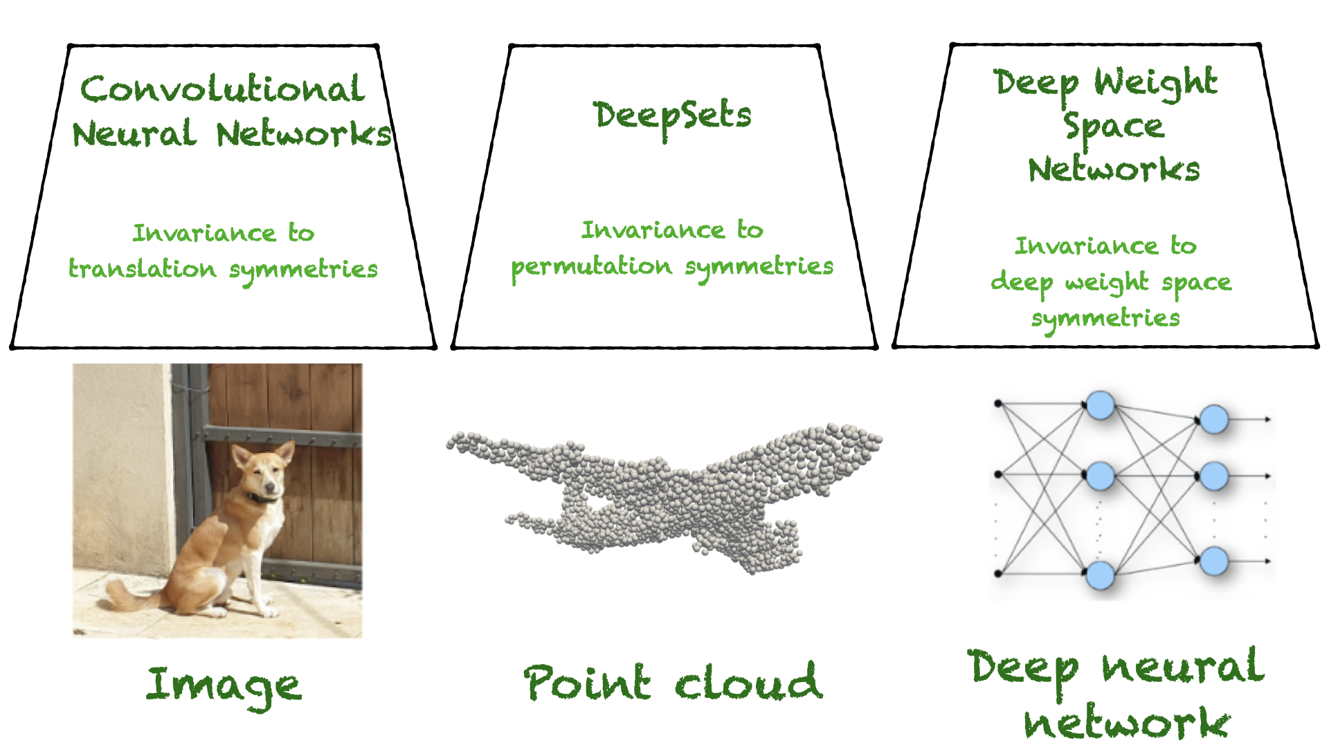

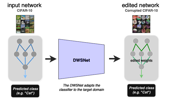
![[W_m, b_l]_{ m in [M],lin[M]}](https://s0.wp.com/latex.php?latex=%5BW_m%2C+b_l%5D_%7B+m+%5Cin+%5BM%5D%2Cl%5Cin%5BM%5D%7D&bg=transparent&fg=000&s=0&c=20201002) . Importantly, in this setup, the weight space is the input space to the (soon-to-be-defined) neural networks.
. Importantly, in this setup, the weight space is the input space to the (soon-to-be-defined) neural networks.

 and
and  cancel each other (assuming an elementwise activation function like ReLU).
 represents permutation matrices. This observation was made more than 30 years ago by Hecht-Nielsen in
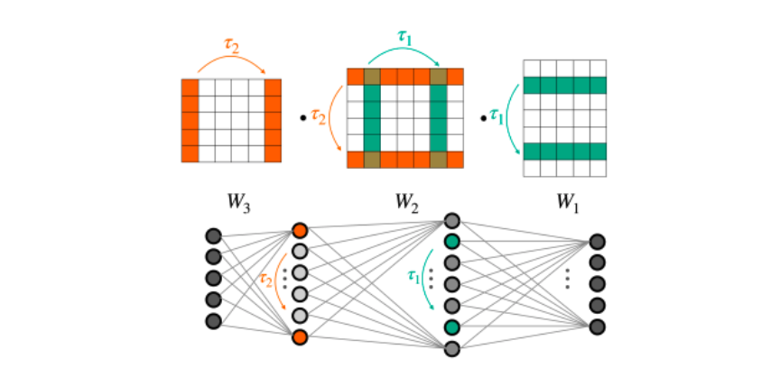
 as a block matrix whose (i,j)-th block is a linear equivariant layer between
  and
and 
 . This block structure is illustrated in Figure 4.
 ? Our paper lists all the possible cases and shows that some of these layers were already characterized in previous work. For example,
  for internal layers was characterized in
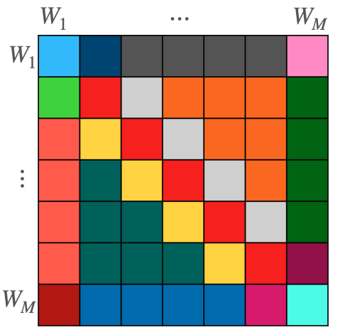
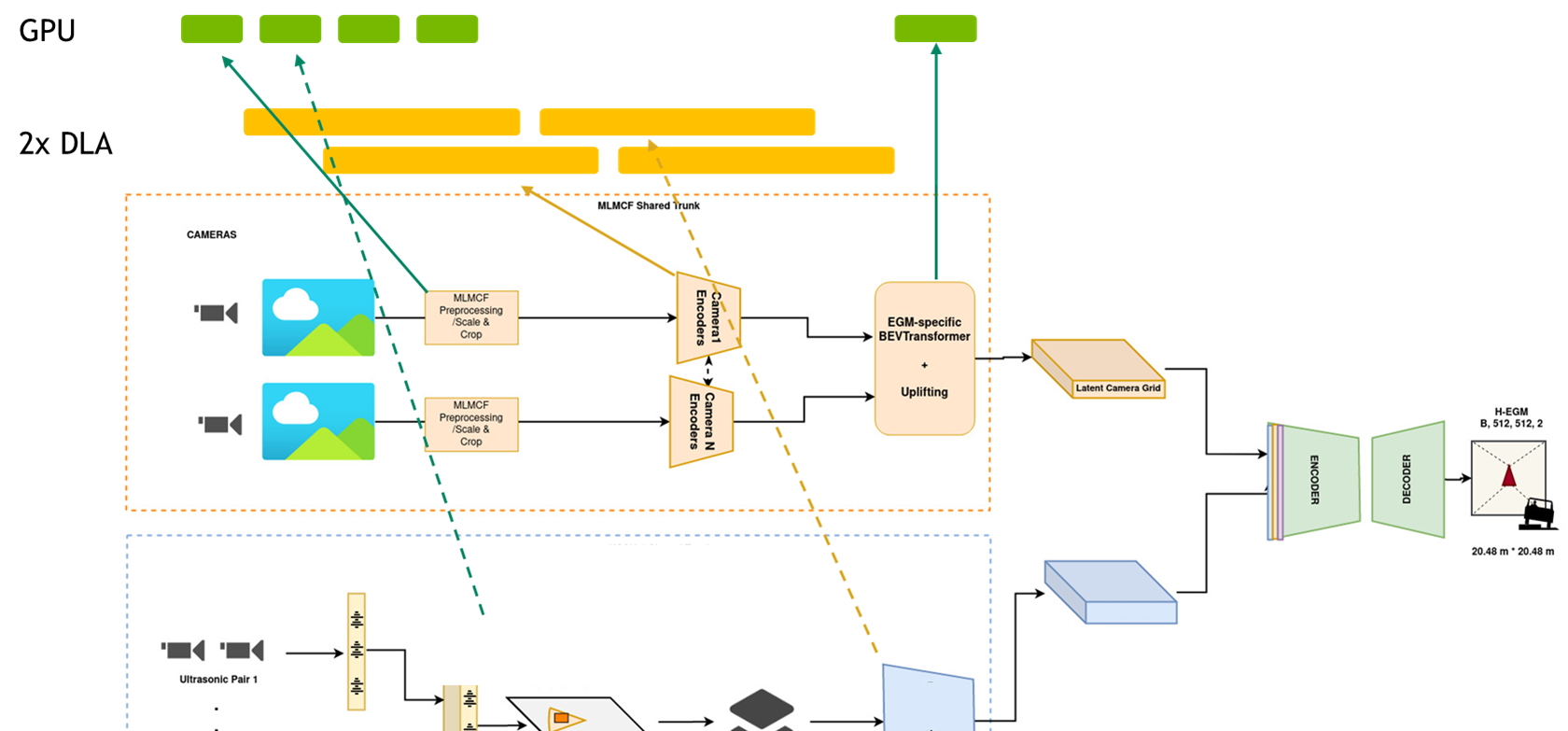
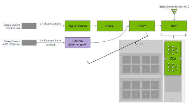
 NVIDIA Jetson Orin is the best-in-class embedded AI platform. The Jetson Orin SoC module has the NVIDIA Ampere architecture GPU at its core but there is a lot…


 On Aug. 29, learn how to create efficient AI models with NVIDIA TAO Toolkit on STM32 MCUs.