As generative AI continues to sweep an increasingly digital, hyperconnected world, NVIDIA founder and CEO Jensen Huang made a thunderous return to SIGGRAPH, the world’s premier computer graphics conference. “The generative AI era is upon us, the iPhone moment if you will,” Huang told an audience of thousands Tuesday during an in-person special address in Read article >
NVIDIA today announced the next-generation NVIDIA GH200 Grace Hopper™ platform — based on a new Grace Hopper Superchip with the world’s first HBM3e processor — built for the era of accelerated computing and generative AI.
NVIDIA and Hugging Face today announced a partnership that will put generative AI supercomputing at the fingertips of millions of developers building large language models (LLMs) and other advanced AI applications.
New Developer Toolkit Introduces Simplified Model Tuning and Deployment on NVIDIA AI Platforms — From PCs and Workstations to Enterprise Data Centers, Public Clouds and NVIDIA DGX CloudLOS …
NVIDIA and global manufacturers today announced powerful new NVIDIA RTX™ workstations designed for development and content creation in the age of generative AI and digitalization.
OVX Servers Feature New NVIDIA GPUs to Accelerate Training and Inference, Graphics-Intensive Workloads; Coming Soon From Dell Technologies, Hewlett Packard Enterprise, Lenovo, Supermicro and …
New Platform Updates, Connections to Adobe Firefly, OpenUSD to RealityKit, Ada-Generation Systems Accelerate Interoperable 3D Workflows and Industrial DigitalizationLOS ANGELES, Aug. 08, 2023 …
Generative AI has introduced a new era in computing, one promising to revolutionize human-computer interaction. At the forefront of this technological marvel…
Generative AI has introduced a new era in computing, one promising to revolutionize human-computer interaction. At the forefront of this technological marvel are large language models (LLMs), empowering enterprises to recognize, summarize, translate, predict, and generate content using large datasets. However, the potential of generative AI for enterprises comes with its fair share of challenges.
Cloud services powered by general-purpose LLMs provide a quick way to get started with generative AI technology. However, these services are often focused on a broad set of tasks and are not trained on domain-specific data, limiting their value for certain enterprise applications. This leads many organizations to build their own solutions—a difficult task—as they must piece together various open-source tools, ensure compatibility, and provide their own support.
NVIDIA NeMo provides an end-to-end platform designed to streamline LLM development and deployment for enterprises, ushering in a transformative age of AI capabilities. NeMo equips you with the essential tools to create enterprise-grade, production-ready custom LLMs. The suite of NeMo tools simplifies the process of data curation, training, and deployment, facilitating the swift development of customized AI applications tailored to each organization’s specific requirements.
For enterprises banking on AI for their business operations, NVIDIA AI Enterprise presents a secure, end-to-end software platform. Combining NeMo with generative AI reference applications and enterprise support, NVIDIA AI Enterprise streamlines the adoption process, paving the way for seamless integration of AI capabilities.
End-to-end platform for production-ready generative AI
The NeMo framework simplifies the path to building customized, enterprise-grade generative AI models by providing end-to-end capabilities and containerized recipes for various model architectures.
Figure 1. End-to-end platform for production-ready generative AI with NeMo
To aid you in creating LLMs, the NeMo framework provides powerful tools:
Data curation
Distributed training at scale
Pretrained models for customization
Accelerated inference
Guardrails
Data curation
In the rapidly evolving landscape of AI, the demand for extensive datasets has become a critical factor in building robust LLMs.
The NeMo framework streamlines the often-complex process of data curation with NeMo Data Curator, which addresses the challenges of curating trillions of tokens in multilingual datasets. Through its scalability, this tool empowers you to effortlessly handle tasks like data download, text extraction, cleaning, filtering, and exact or fuzzy deduplication.
By harnessing the power of cutting-edge technologies, including Message-Passing Interface (MPI), Dask, and Redis Cluster, Data Curator can scale data-curation processes across thousands of compute cores, significantly reducing manual efforts and accelerating the development workflow.
One of the key benefits of Data Curator lies in its deduplication feature. By ensuring that LLMs are trained on unique documents, you can avoid redundant data and potentially achieve substantial cost savings during the pretraining phase. This not only streamlines the model development process but also optimizes AI investments for organizations, making AI development more accessible and cost-effective.
Data Curator comes packaged in the NeMo training container available through NGC.
Distributed training at scale
Training billion-parameter LLM models from scratch presents unique challenges of acceleration and scale. The process demands massive, distributed computing power, clusters of acceleration-based hardware and memory, reliable and scalable machine learning (ML) frameworks, and fault-tolerant systems.
At the heart of the NeMo framework lies the unification of distributed training and advanced parallelism. NeMo expertly uses GPU resources and memory across nodes, leading to groundbreaking efficiency gains. By dividing the model and training data, NeMo enables seamless multi-node and multi-GPU training, significantly reducing training time and enhancing overall productivity.
A standout feature of NeMo is its incorporation of various parallelism techniques:
Data parallelism
Tensor parallelism
Pipeline parallelism
Sequence parallelism
Sparse attention reduction (SAR).
These techniques work in tandem to optimize the training process, thereby maximizing resource usage and bolstering performance.
NeMo also offers an array of precision options:
FP32/TF32
BF16
FP8
Groundbreaking innovations like FlashAttention and Rotary Positional Embedding (RoPE) cater to long sequence-length tasks. Attention with Linear Biases (ALiBi), gradient and partial checkpointing, and the Distributed Adam Optimizer further elevate model performance and speed.
Pretrained models for customization
While some generative AI use cases require training from scratch, more and more organizations are using pretrained models to jump-start their effort when building customized LLMs.
One of the most significant benefits of pretrained models is the savings in time and resources. By skipping the data collection and cleaning phases required to pre-train the generic LLM, you can focus on fine-tuning models to their specific needs, accelerating the time to the final solution. Moreover, the burden of infrastructure setup and model training is greatly reduced, as pretrained models come with pre-existing knowledge, ready to be customized.
Thousands of open-source models are also available on hubs like GitHub, Hugging Face, and others, so you have choices when it comes to which model to start with. Accuracy is one of the more common measurements to evaluate pretrained models, but there are also other considerations:
Size
Cost to fine-tune
Latency
Memory constraints
Commercial licensing options
With NeMo, you can now access a wide range of pretrained models, from NVIDIA and popular open-source repositories like Falcon AI, Llama-2, and MPT 7B.
NeMo models are optimized for inference, making them ideal for production use cases. With the ability to deploy these models in real-world applications, you can drive transformative outcomes and unlock the full potential of AI for your organizations.
Model customization
Customization of ML models is rapidly evolving to accommodate the unique needs of businesses and industries. The NeMo framework offers an array of techniques to refine generic, pretrained LLMs for specialized use cases. Through these diverse customization options, NeMo offers wide-ranging flexibility that is crucial in meeting varying business requirements.
Prompt engineeringis an efficient customization method that makes it possible to use pretrained LLMs on many downstream tasks without needing to tune the pretrained models’ parameters. The goal of prompt engineering is to design and optimize prompts that are specific and clear enough to elicit the desired output from the model.
P-tuning and prompt tuning are parameter-efficient fine-tuning (PETF) techniques that use clever optimizations to selectively update only a few parameters of the LLM. As implemented in NeMo, new tasks can be added to a model without overwriting or disrupting previous tasks for which the model has already been tuned.
NeMo has optimized its p-tuning methods for use on multi-GPU and multi-node environments enabling accelerated training. NeMo p-tuning also supports an ‘early stop’ mechanism that identifies when a model has converged to the point when further training won’t improve accuracy much. It then stops the training job. This technique reduces the time and resources needed to customize models.
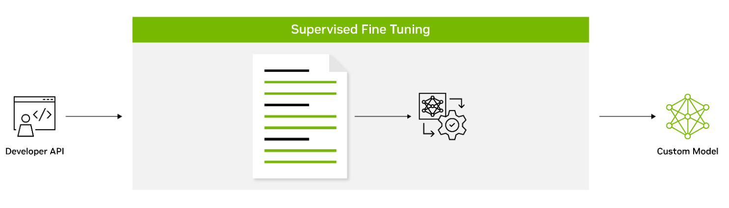
Figure 2. Supervised fine-tuning with labeled datasets
Supervised fine-tuning(SFT) involves fine-tuning a model’s parameters using labeled data. Also known as instruction tuning, this form of customization is typically conducted post-pretraining. It provides the advantage of using state-of-the-art models without the need for initial training, thus lowering computational costs and reducing data collection requirements.
Adapters introduce small feedforward layers in between the model’s core layers. These adapter layers are then fine-tuned for specific downstream tasks, providing a level of customization that is unique to the requirements of the task at hand.
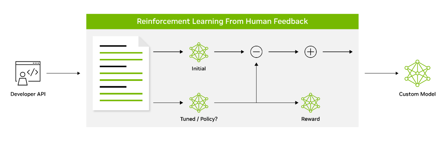
Figure 3. Aligning LLM behavior with human preferences using reinforcement learning
Reinforcement learning from human feedback (RLHF) employs a three-stage fine-tuning process. The model adapts its behavior based on feedback, encouraging a better alignment with human values and preferences. This makes RLHF a powerful tool for creating models that resonate with human users.
AliBi enables transformer models to process longer sequences at inference time than they were trained on. This is particularly useful in scenarios where the information to be processed is lengthy or complex.
NeMo Guardrails helps ensure that smart applications powered by LLMs are accurate, appropriate, on-topic, and secure. NeMo Guardrails is available as open source and includes all the code, examples, and documentation businesses need for adding safety to AI apps that generate text. NeMo Guardrails works with NeMo as well as all LLMs, including OpenAI’s ChatGPT.
Accelerated inference
Seamlessly integrating with NVIDIA Triton Inference Server, NeMo significantly accelerates the inference process, delivering exceptional accuracy, low latency, and high throughput. This integration facilitates secure and efficient deployments ranging from a single GPU to large-scale, multi-node GPUs, while adhering to stringent safety and security requirements.
NVIDIA Triton empowers NeMo to streamline and standardize generative AI inference. This enables teams to deploy, run, and scale trained ML or deep learning (DL) models from any framework on any GPU- or CPU-based infrastructure. This high level of flexibility provides you with the freedom to choose the most suitable framework for your AI research and data science projects without compromising production deployment flexibility.
Guardrails
As part of the NVIDIA AI Enterprise software suite, NeMo enables organizations to deploy production-ready generative AI with confidence. Organizations can take advantage of long-term branch support for up to 3 years, ensuring seamless operations and stability. Regular Common Vulnerabilities and Exposures (CVE) scans, security notifications, and timely patches enhance security, while API stability simplifies updates.
NVIDIA AI Enterprise support services are included with the purchase of the NVIDIA AI Enterprise software suite. We provide direct access to NVIDIA AI experts, defined service-level agreements, and control of upgrade and maintenance schedules with long-term support options.
Powering enterprise-grade generative AI
As part of NVIDIA AI Enterprise 4.0, NeMo offers seamless compatibility across multiple platforms, including the cloud, data centers, and now, NVIDIA RTX-powered workstations and PCs. This enables a true develop-once-and-deploy-anywhere experience, eliminates the complexities of integration, and maximizes operational efficiency.
NeMo has already gained significant traction among forward-thinking organizations looking to build custom LLMs. Writer and Korea Telecom have embraced NeMo, leveraging its capabilities to drive their AI-driven initiatives.
The unparalleled flexibility and support provided by NeMo opens a world of possibilities for businesses, enabling them to design, train, and deploy sophisticated LLM solutions tailored to their specific needs and industry verticals. By partnering with NVIDIA AI Enterprise and integrating NeMo into their workflows, your organizations can unlock new avenues of growth, derive valuable insights, and deliver cutting-edge AI-powered applications to customers, clients, and employees alike.
Get started with NVIDIA NeMo
NVIDIA NeMo has emerged as a game-changing solution, bridging the gap between the immense potential of generative AI and the practical realities faced by enterprises. A comprehensive platform for LLM development and deployment, NeMo empowers businesses to leverage AI technology efficiently and cost-effectively.
With these powerful capabilities, enterprises can integrate AI into their operations, streamlining processes, enhancing decision-making capabilities, and unlocking new avenues for growth and success.
Learn more about NVIDIA NeMo and how it helps enterprises build production-ready generative AI.
The latest developments in large language model (LLM) scaling laws have shown that when scaling the number of model parameters, the number of tokens used for…
The latest developments in large language model (LLM) scaling laws have shown that when scaling the number of model parameters, the number of tokens used for training should be scaled at the same rate. The Chinchilla and LLaMA models have validated these empirically derived laws and suggest that previous state-of-the-art models have been under-trained regarding the total number of tokens used during pretraining.
Considering these recent developments, it’s apparent that LLMs need larger datasets, more than ever.
However, despite this need, most software and tools developed to create massive datasets for training LLMs are not publicly released or scalable. This requires LLM developers to build their own tools to curate large language datasets.
To meet this growing need for large datasets, we have developed and released the NeMo Data Curator: a scalable data-curation tool that enables you to curate trillion-token multilingual datasets for pretraining LLMs.
Applying these modules to your datasets helps reduce the burden of combing through unstructured data sources. Through document-level deduplication, you can ensure that models are trained on unique documents, potentially leading to greatly reduced pretraining costs.
In this post, we provide an overview of each module in Data Curator and demonstrate that they offer linear scaling to more than 1000 CPU cores. To validate the data curated, we also show that using documents it processes from Common Crawl for pretraining provides significant downstream task improvement over using raw downloaded documents.
Data-curation pipeline
This tool enables you to download data and extract, clean, deduplicate, and filter documents at scale. Figure 1 shows a typical LLM data-curation pipeline that can be implemented. In the following sections, we briefly describe the implementation of each of these modules available.
Figure 1. A common LLM data-curation pipeline for datasets like Common Crawl that can be implemented with the modules available within the Data Curator
Download and text extraction
The starting point for preparing custom pretraining datasets for many LLM practitioners is a list of URLs that point to data files or websites that contain content of interest for LLM pretraining.
Data Curator enables you to download pre-crawled web pages from data repositories such as Common Crawl, Wikidumps, and ArXiv and to extract the relevant text to JSONL files at scale. Data Curator also provides you with the flexibility of supplying your own download and extraction functions to process datasets from a variety of sources. Using a combination of MPI and Python Multiprocessing, thousands of asynchronous download and extraction workers can be launched at runtime across many compute nodes.
Text reformatting and cleaning
Upon downloading and extracting text from documents, a common step is to fix all Unicode-related errors that can be introduced when text data are not properly decoded during extraction. Data Curator uses the Fixes Text For You library (ftfy) to fix all Unicode-related errors. Cleaning also helps to normalize the text, which results in a higher recall when performing document deduplication.
Document-level deduplication
When downloading data from massive web-crawl sources such as Common Crawl, it’s common to encounter both documents that are exact duplicates and documents with high similarity (that is, near duplicates). Pretraining LLMs with repeated documents can lead to poor generalization and a lack of diversity during text generation.
We provide exact and fuzzy deduplication utilities to remove duplicates from text data. The exact deduplication utility computes a 128-bit hash of each document, groups documents by their hashes into buckets, selects one document per bucket, and removes the remaining exact duplicates within the bucket.
The fuzzy-deduplication utility uses a MinHashLSH-based approach where MinHashes are computed for each document, and then documents are grouped using the locality-sensitive property of min-wise hashing. After documents are grouped into buckets, similarities are computed between documents within each bucket to check for potential false positives created during MinHashLSH.
For both deduplication utilities, Data Curator uses a Redis Cluster distributed across compute nodes to implement a distributed dictionary for clustering documents into buckets. The scalable design and gossip protocol implemented by the Redis Cluster enables efficient scaling of deduplication workloads to many compute nodes.
Document-level quality filtering
In addition to containing a significant fraction of duplicate documents, data from web-crawl sources such as Common Crawl often tend to include many documents with informal prose. This includes, for example, many URLs, symbols, boilerplate content, ellipses, or repeating substrings. They can be considered low-quality content from a language-modeling perspective.
While it’s been shown that diverse LLM pretraining datasets lead to improved downstream performance, a significant quantity of low-quality documents can hinder performance. Data Curator provides you with a highly configurable document-filtering utility that enables you to apply custom heuristic filters at scale to your corpora. The tool also includes implementations of language-data filters (both classifier and heuristic-based) that have been shown to improve overall data quality and downstream task performance when applied to web-crawl data.
Scaling to many compute cores
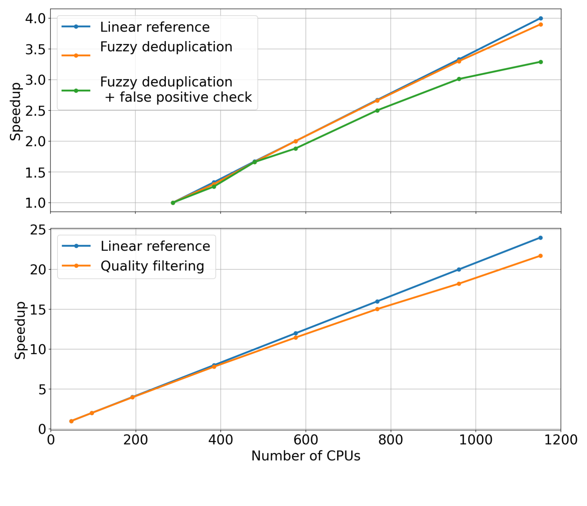
To demonstrate the scaling capabilities of the different modules available within Data Curator, we used them to prepare a small dataset consisting of approximately 40B tokens. This involved running the previously described data-curation pipeline on 5 TB of Common Crawl WARC files.
For each pipeline stage, we fixed the input dataset size while linearly increasing the number of CPU cores used to scale the data curation modules (that is, strong scaling). We then measured the speedup for each module. The measured speedups for the quality-filtering and fuzzy-deduplication modules are shown in Figure 2.
Examining the trends of the measurements, it’s apparent that these modules can reach substantial speedups when increasing the number of CPU cores used for distributing the data curation workloads. Compared to the linear reference (orange curve), we observe that both modules are able to achieve considerable speedup when using up to 1,000 CPUs or more.
Figure 2. Measured speedup for the fuzzy-deduplication and quality-filtering modules within Data Curator
Curated pretraining data results in improved model downstream performance
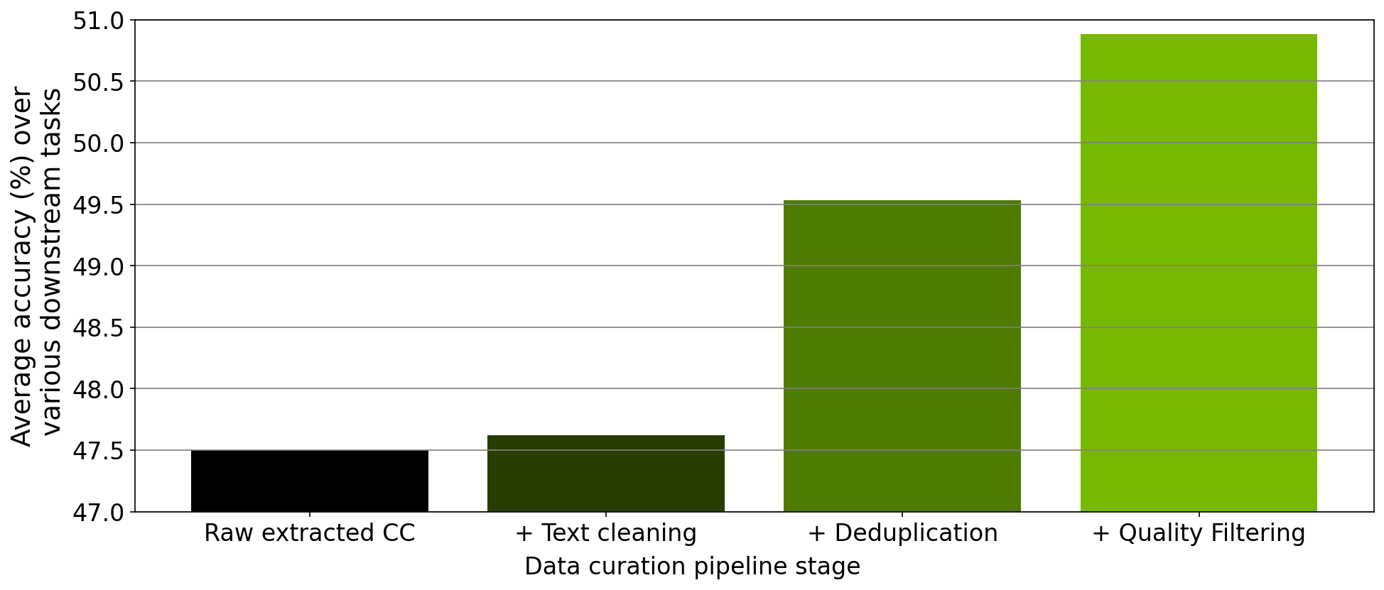
In addition to verifying the scaling of each module, we also performed an ablation study on the data curated from each step of the data-curation pipeline implemented within the tool. Starting from a downloaded Common Crawl snapshot, we trained a 357M parameter GPT model on 78M tokens curated from this snapshot after extraction, cleaning, deduplication, and filtering.
After each pretraining experiment, we evaluated the model across the RACE-High, PiQA, Winogrande, and Hellaswag tasks in a zero-shot setting. Figure 3 shows that the results of our ablation experiments averaged over all four tasks. As the data progresses through the different stages of the pipeline, the average over all four tasks increases significantly, indicating improved data quality.
Figure 3. Results of dataset ablation tests for a 357M parameter model trained on data generated from each stage of the processing pipeline within NeMo Data Curator
Curating a 2T token dataset with NeMo Data Curator
Recently, the NVIDIA NeMo service started providing early-access users with the opportunity to customize an NVIDIA-trained 43B-parameter multilingual large foundation model. To pretrain this foundation model, we prepared a dataset consisting of 2T tokens that included 53 natural languages originating from a variety of diverse domains as well as 37 different programming languages.
Curating this large dataset required applying our data-curation pipeline implemented within Data Curator to a total of 8.7 TB of text data on a CPU cluster of more than 6K CPUs. Pretraining the 43B foundation model on 1.1T of these tokens resulted in a state-of-the-art LLM that’s currently being used by NVIDIA customers for their LLM needs.
Conclusion
To meet the growing demands for curating pretraining datasets for LLMs, we have released Data Curator as part of the NeMo framework. We have demonstrated that the tool curates high-quality data that leads to improved LLM downstream performance. Further, we have shown that each data-curation module available within Data Curator can scale to use thousands of CPU cores. We anticipate that this tool will significantly benefit LLM developers attempting to build pretraining datasets.
Developing extended reality (XR) applications can be extremely challenging. Users typically start with a template project and adhere to pre-existing packaging…
Developing extended reality (XR) applications can be extremely challenging. Users typically start with a template project and adhere to pre-existing packaging templates for deploying an app to a headset. This approach creates a distinct bottleneck in the asset iteration pipeline. Updating assets inside an XR experience becomes completely dependent on how fast the developer can build, package, and deploy a new executable.
The new spatial framework in NVIDIA Omniverse helps tackle these challenges with Universal Scene Description, known as OpenUSD, and NVIDIA RTX-enabled ray tracing. This marks the world’s first fully ray-traced XR experience, enabling you to view every reflection, soft shadow, limitless light, and dynamic change to geometry in your scene.
You can now fully ray trace massive, complex, full fidelity design data sets with millions of polygons, physical materials, and accurate lighting. Experience the data sets in an immersive environment without requiring additional time for data preparation.
Enabling immersive workflows with OpenUSD
OpenUSD ensures that scene editing remains nondestructive, enabling seamless interactions between different tools and ecosystems. Omniverse renders and presents the USD data on disk, so users can iterate on that data at any cadence and see the XR view of the asset updated in real time.
As a result, users can experience applications immersively at any point in the pipeline, drastically reducing friction and increasing iteration speeds. Users can even integrate XR in existing pipelines—it is no longer time-intensive to implement.
Key features of the spatial framework include:
New tools for adding immersive experiences and basic XR functionality. This streamlines workflows for design reviews and factory planning.
Connects RTX ray tracing and Omniverse to SteamVR, OpenXR, and NVIDIA CloudXR.
Support for spatial computing platforms and headsets.Omniverse users can build USD stages that are compatible with other OpenUSD-based spatial computing platforms such as AR Kit and RealityKit. Plus, new support for the Khronos Group OpenXR open standard expands Omniverse-developer experiences to more headsets from manufacturers such as HTC Vive, Magic Leap, and Varjo.
“The NVIDIA release of Omniverse Kit with OpenXR and Magic Leap 2 support is an important milestone for enterprise AR,” said Jade Meskill, VP Product at Magic Leap. “Enterprise users can now render and stream immersive, full-scale digital twins from Omniverse to Magic Leap 2 with groundbreaking visual quality.”
Placing photorealistic digital twins based on full fidelity design data in the real world with accurate lighting and reflections is a must-have for demanding enterprise applications, added Meskill. “We are delighted by the strong partnership between the NVIDIA and Magic Leap engineering teams that pioneered key technical advancements in visual quality.”
Integrating XR into existing 3D workflows
Omniverse application developers can now easily integrate XR into 3D workflows. The new spatial framework in Omniverse enables real-time, immersive visualization for 3D scenes. You can also incorporate XR functionalities, such as teleporting, manipulating, and navigating, into existing pipelines.
Using the spatial framework, you can view working assets in mixed reality, or totally immersively, across devices. NVIDIA CloudXR enables a completely untethered experience with the same level of fidelity that only desktop compute can provide.
You can also use specific extensions without downloading an entire application, enabling simpler and more modular workflows. Automatic user interface optimizations improve the speed and productivity of applications to provide smoother playbacks.
In addition, you can deploy custom XR applications and design user interfaces for specific workflows, such as collaborative product design review and factory planning.
RTX-powered immersive experiences on industry-leading headsets
With Omniverse Kit 105, you can create assets with ultimate immersion and realism and build apps that are incredibly realistic, with full fidelity, geometry, and materials.
For example, Kit 105 can drive the retinal resolution Quad View rendering for the Varjo XR-3, the industry’s highest resolution mixed-reality headset. The renderer produces two high-resolution views and two lower resolution views, which are then composited by the device to provide an unparalleled level of fidelity and immersion within the VR experience.
“Real-time ray tracing is the holy grail of 3D visualization,” explains Marcus Olsson, director of Software Partnerships at Varjo. “The graphical and computing demands made it impossible to render true-to-life immersive scenes like these—until now. With NVIDIA Omniverse and Varjo XR-3, users can unlock real-time ray tracing for mixed reality environments due to the combination of a powerful multi-GPU setups and Varjo’s photorealistic visual fidelity.”
The Quad View renders a staggering 15 million pixels, unlocking new levels of visual fidelity in XR. Teams seeking to leverage retinal resolution Quad View rendering should use a multi-GPU setup powered by the latest NVIDIA RTX 6000 Ada Generation graphics cards to provide seamless rendering and optimal performance for the Varjo XR-3 headset.
Start building immersive experiences and applications with Omniverse
Ready to start building XR into applications and creating immersive experiences using Omniverse Kit 105? The spatial framework is available now in the Omniverse Extension Library under VR Experience. Add the extension to your Kit app and the Tablet AR and VR panels will be ready to use. Omni.UI is also implemented in the framework, so tools and interfaces you develop for desktop can be used while in a headset.
USD Composer provides a good place to test immersive experiences in Omniverse. USD Composer is a reference application in Omniverse where you can easily open and craft a USD stage. To get started, install USD Composer from the Omniverse Launcher. In the Window -> Rendering menu, find VR and Tablet AR. If you’re working with another user, you can leverage the USD Composer multi-user workflow to work immersively together in real time. Get started building your own XR experience in Omniverse.

 Generative AI has introduced a new era in computing, one promising to revolutionize human-computer interaction. At the forefront of this technological marvel…
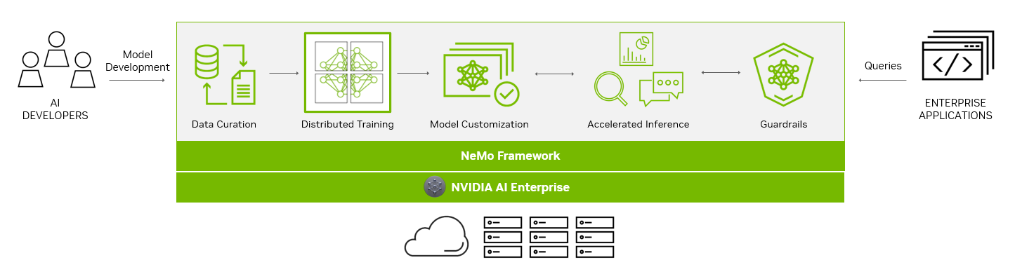
 The latest developments in large language model (LLM) scaling laws have shown that when scaling the number of model parameters, the number of tokens used for…
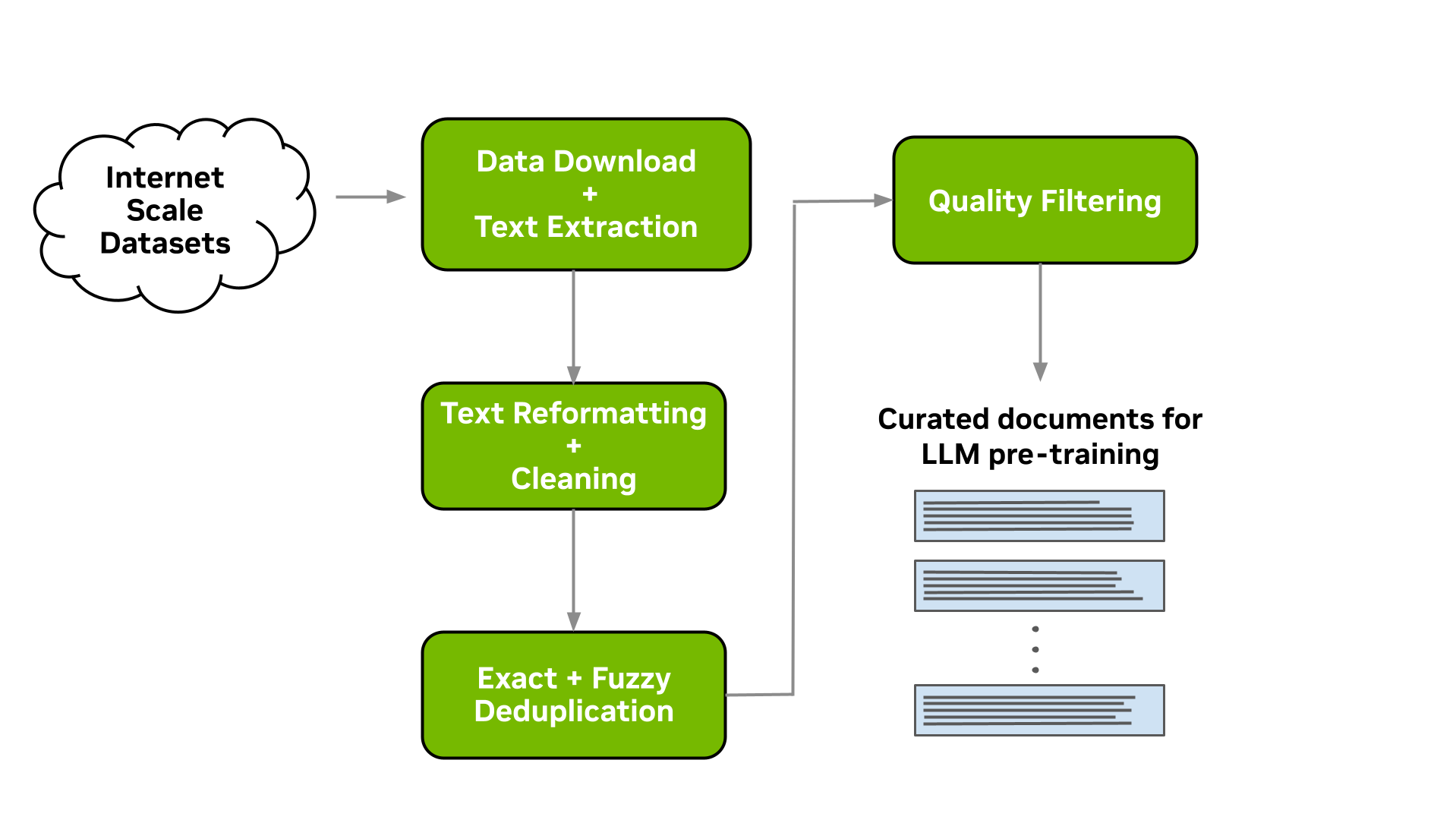
 Developing extended reality (XR) applications can be extremely challenging. Users typically start with a template project and adhere to pre-existing packaging…