

Deep learning has recently made tremendous progress in a wide range of problems and applications, but models often fail unpredictably when deployed in unseen domains or distributions. Source-free domain adaptation (SFDA) is an area of research that aims to design methods for adapting a pre-trained model (trained on a “source domain”) to a new “target domain”, using only unlabeled data from the latter.
Designing adaptation methods for deep models is an important area of research. While the increasing scale of models and training datasets has been a key ingredient to their success, a negative consequence of this trend is that training such models is increasingly computationally expensive, out of reach for certain practitioners and also harmful for the environment. One avenue to mitigate this issue is through designing techniques that can leverage and reuse already trained models for tackling new tasks or generalizing to new domains. Indeed, adapting models to new tasks is widely studied under the umbrella of transfer learning.
SFDA is a particularly practical area of this research because several real-world applications where adaptation is desired suffer from the unavailability of labeled examples from the target domain. In fact, SFDA is enjoying increasing attention [1, 2, 3, 4]. However, albeit motivated by ambitious goals, most SFDA research is grounded in a very narrow framework, considering simple distribution shifts in image classification tasks.
In a significant departure from that trend, we turn our attention to the field of bioacoustics, where naturally-occurring distribution shifts are ubiquitous, often characterized by insufficient target labeled data, and represent an obstacle for practitioners. Studying SFDA in this application can, therefore, not only inform the academic community about the generalizability of existing methods and identify open research directions, but can also directly benefit practitioners in the field and aid in addressing one of the biggest challenges of our century: biodiversity preservation.
In this post, we announce “In Search for a Generalizable Method for Source-Free Domain Adaptation”, appearing at ICML 2023. We show that state-of-the-art SFDA methods can underperform or even collapse when confronted with realistic distribution shifts in bioacoustics. Furthermore, existing methods perform differently relative to each other than observed in vision benchmarks, and surprisingly, sometimes perform worse than no adaptation at all. We also propose NOTELA, a new simple method that outperforms existing methods on these shifts while exhibiting strong performance on a range of vision datasets. Overall, we conclude that evaluating SFDA methods (only) on the commonly-used datasets and distribution shifts leaves us with a myopic view of their relative performance and generalizability. To live up to their promise, SFDA methods need to be tested on a wider range of distribution shifts, and we advocate for considering naturally-occurring ones that can benefit high-impact applications.
Distribution shifts in bioacoustics
Naturally-occurring distribution shifts are ubiquitous in bioacoustics. The largest labeled dataset for bird songs is Xeno-Canto (XC), a collection of user-contributed recordings of wild birds from across the world. Recordings in XC are “focal”: they target an individual captured in natural conditions, where the song of the identified bird is at the foreground. For continuous monitoring and tracking purposes, though, practitioners are often more interested in identifying birds in passive recordings (“soundscapes”), obtained through omnidirectional microphones. This is a well-documented problem that recent work shows is very challenging. Inspired by this realistic application, we study SFDA in bioacoustics using a bird species classifier that was pre-trained on XC as the source model, and several “soundscapes” coming from different geographical locations — Sierra Nevada (S. Nevada); Powdermill Nature Reserve, Pennsylvania, USA; Hawai’i; Caples Watershed, California, USA; Sapsucker Woods, New York, USA (SSW); and Colombia — as our target domains.
This shift from the focalized to the passive domain is substantial: the recordings in the latter often feature much lower signal-to-noise ratio, several birds vocalizing at once, and significant distractors and environmental noise, like rain or wind. In addition, different soundscapes originate from different geographical locations, inducing extreme label shifts since a very small portion of the species in XC will appear in a given location. Moreover, as is common in real-world data, both the source and target domains are significantly class imbalanced, because some species are significantly more common than others. In addition, we consider a multi-label classification problem since there may be several birds identified within each recording, a significant departure from the standard single-label image classification scenario where SFDA is typically studied.
 |
| Illustration of the “focal → soundscapes” shift. In the focalized domain, recordings are typically composed of a single bird vocalization in the foreground, captured with high signal-to-noise ratio (SNR), though there may be other birds vocalizing in the background. On the other hand, soundscapes contain recordings from omnidirectional microphones and can be composed of multiple birds vocalizing simultaneously, as well as environmental noises from insects, rain, cars, planes, etc. |
| Audio files |
Focal domain |
Soundscape domain1 |
||
| Spectogram images |  |
 |
| Illustration of the distribution shift from the focal domain (left) to the soundscape domain (right), in terms of the audio files (top) and spectrogram images (bottom) of a representative recording from each dataset. Note that in the second audio clip, the bird song is very faint; a common property in soundscape recordings where bird calls aren’t at the “foreground”. Credits: Left: XC recording by Sue Riffe (CC-BY-NC license). Right: Excerpt from a recording made available by Kahl, Charif, & Klinck. (2022) “A collection of fully-annotated soundscape recordings from the Northeastern United States” [link] from the SSW soundscape dataset (CC-BY license). |
State-of-the-art SFDA models perform poorly on bioacoustics shifts
As a starting point, we benchmark six state-of-the-art SFDA methods on our bioacoustics benchmark, and compare them to the non-adapted baseline (the source model). Our findings are surprising: without exception, existing methods are unable to consistently outperform the source model on all target domains. In fact, they often underperform it significantly.
As an example, Tent, a recent method, aims to make models produce confident predictions for each example by reducing the uncertainty of the model’s output probabilities. While Tent performs well in various tasks, it doesn’t work effectively for our bioacoustics task. In the single-label scenario, minimizing entropy forces the model to choose a single class for each example confidently. However, in our multi-label scenario, there’s no such constraint that any class should be selected as being present. Combined with significant distribution shifts, this can cause the model to collapse, leading to zero probabilities for all classes. Other benchmarked methods like SHOT, AdaBN, Tent, NRC, DUST and Pseudo-Labelling, which are strong baselines for standard SFDA benchmarks, also struggle with this bioacoustics task.
 |
| Evolution of the test mean average precision (mAP), a standard metric for multilabel classification, throughout the adaptation procedure on the six soundscape datasets. We benchmark our proposed NOTELA and Dropout Student (see below), as well as SHOT, AdaBN, Tent, NRC, DUST and Pseudo-Labelling. Aside from NOTELA, all other methods fail to consistently improve the source model. |
Introducing NOisy student TEacher with Laplacian Adjustment (NOTELA)
Nonetheless, a surprisingly positive result stands out: the less celebrated Noisy Student principle appears promising. This unsupervised approach encourages the model to reconstruct its own predictions on some target dataset, but under the application of random noise. While noise may be introduced through various channels, we strive for simplicity and use model dropout as the only noise source: we therefore refer to this approach as Dropout Student (DS). In a nutshell, it encourages the model to limit the influence of individual neurons (or filters) when making predictions on a specific target dataset.
DS, while effective, faces a model collapse issue on various target domains. We hypothesize this happens because the source model initially lacks confidence in those target domains. We propose improving DS stability by using the feature space directly as an auxiliary source of truth. NOTELA does this by encouraging similar pseudo-labels for nearby points in the feature space, inspired by NRC’s method and Laplacian regularization. This simple approach is visualized below, and consistently and significantly outperforms the source model in both audio and visual tasks.
 |
 |
| NOTELA in action. The audio recordings are forwarded through the full model to obtain a first set of predictions, which are then refined through Laplacian regularization, a form of post-processing based on clustering nearby points. Finally, the refined predictions are used as targets for the noisy model to reconstruct. |
Conclusion
The standard artificial image classification benchmarks have inadvertently limited our understanding of the true generalizability and robustness of SFDA methods. We advocate for broadening the scope and adopt a new assessment framework that incorporates naturally-occurring distribution shifts from bioacoustics. We also hope that NOTELA serves as a robust baseline to facilitate research in that direction. NOTELA’s strong performance perhaps points to two factors that can lead to developing more generalizable models: first, developing methods with an eye towards harder problems and second, favoring simple modeling principles. However, there is still future work to be done to pinpoint and comprehend existing methods’ failure modes on harder problems. We believe that our research represents a significant step in this direction, serving as a foundation for designing SFDA methods with greater generalizability.
Acknowledgements
One of the authors of this post, Eleni Triantafillou, is now at Google DeepMind. We are posting this blog post on behalf of the authors of the NOTELA paper: Malik Boudiaf, Tom Denton, Bart van Merriënboer, Vincent Dumoulin*, Eleni Triantafillou* (where * denotes equal contribution). We thank our co-authors for the hard work on this paper and the rest of the Perch team for their support and feedback.
1Note that in this audio clip, the bird song is very faint; a common property in soundscape recordings where bird calls aren’t at the “foreground”. ↩
 On July 26, connect with CUDA product team experts on the latest NVIDIA CUDA Toolkit 12.
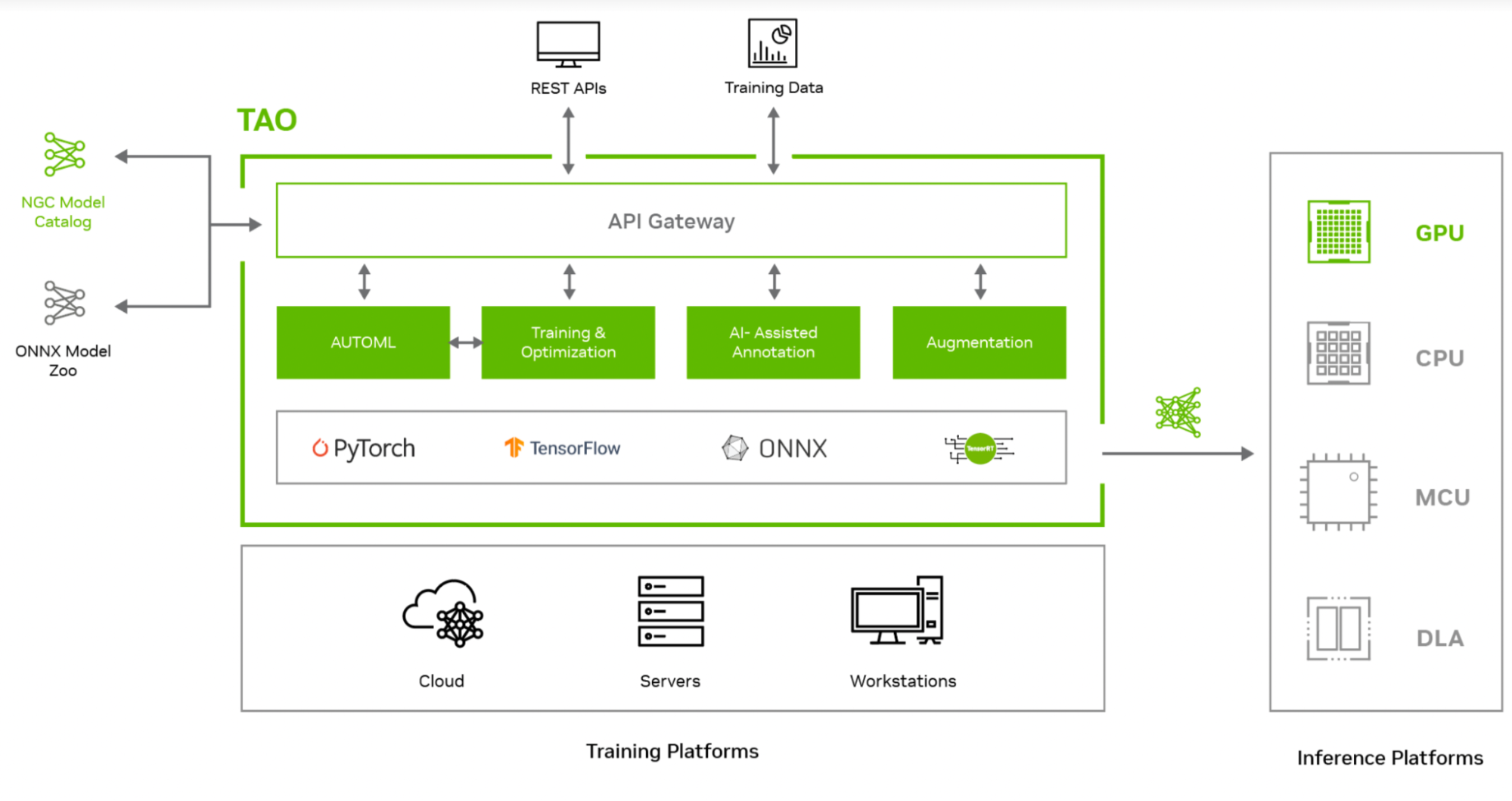
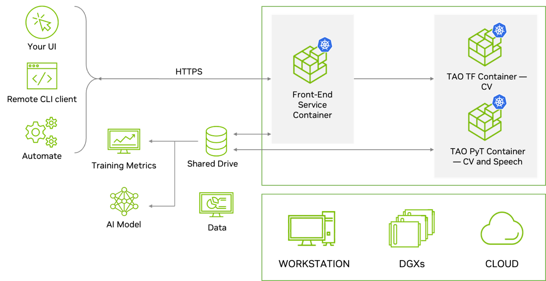
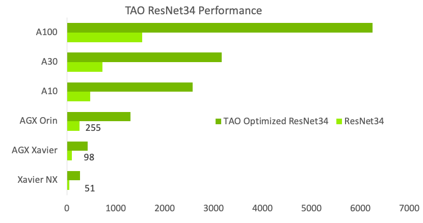
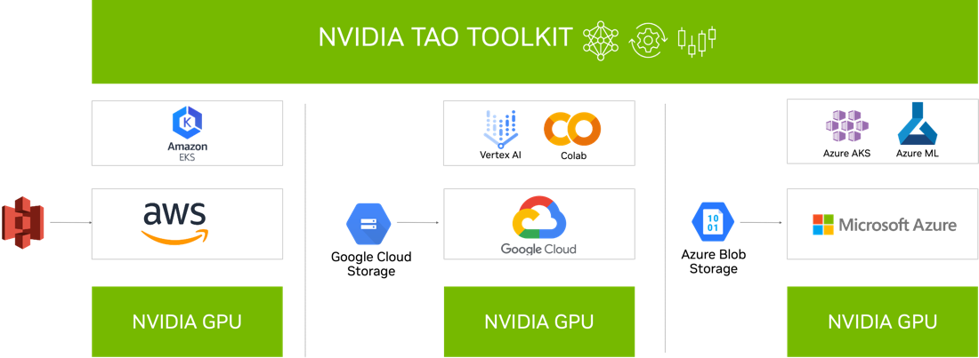
  NVIDIA TAO Toolkit provides a low-code AI framework to accelerate vision AI model development suitable for all skill levels, from novice beginners to expert…
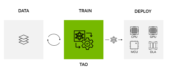

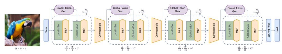
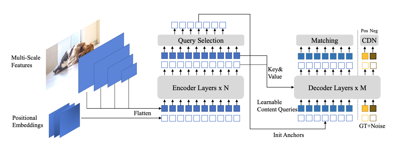
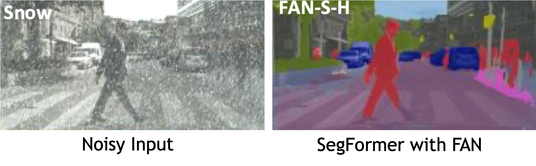
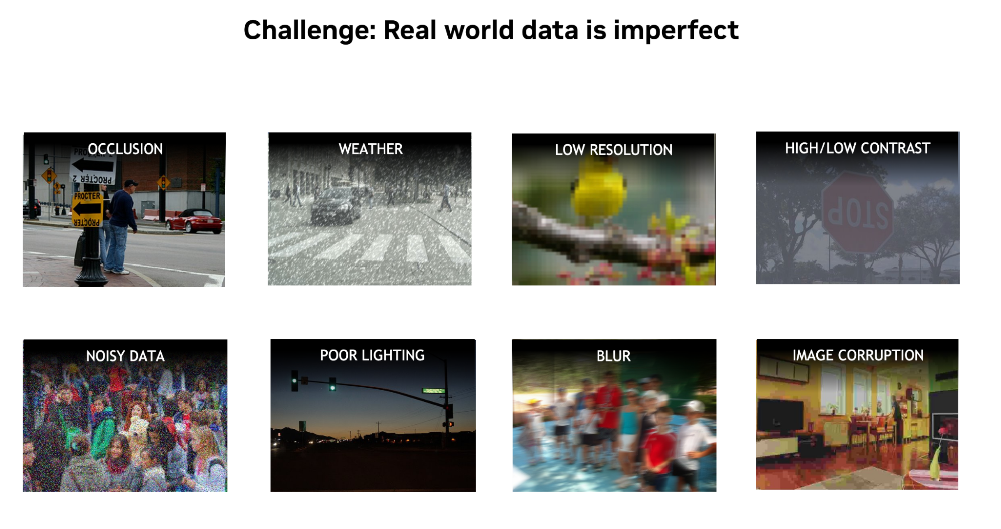
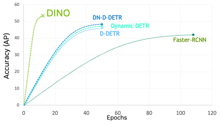
 Vision Transformers (ViTs) are taking computer vision by storm, offering incredible accuracy, robust solutions for challenging real-world scenarios, and…
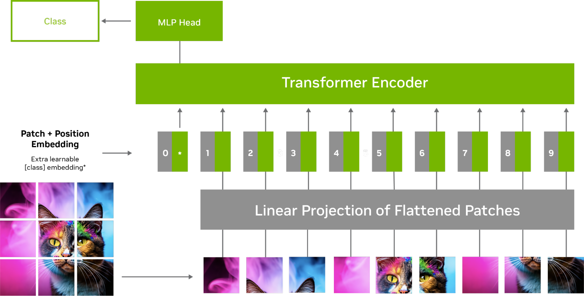
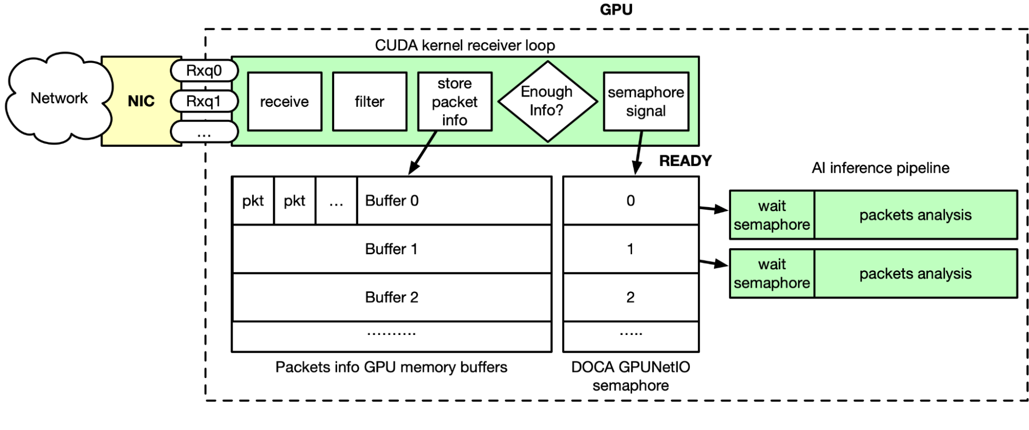
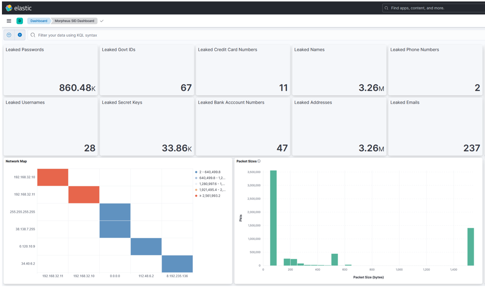
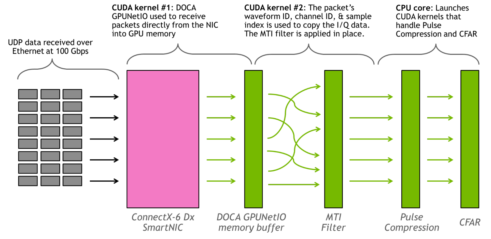
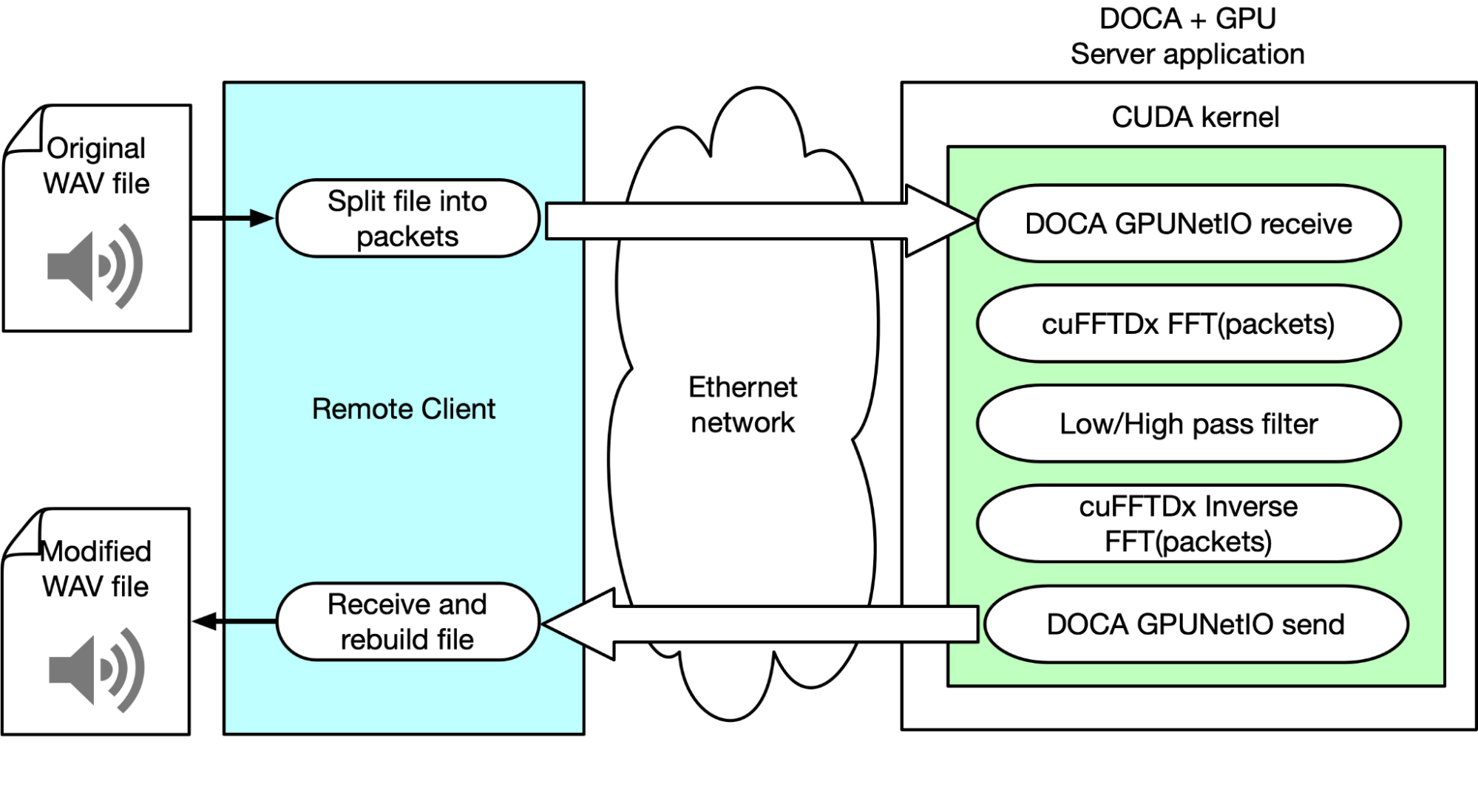
 Real-time processing of network traffic can be leveraged by the high degree of parallelism GPUs offer. Optimizing packet acquisition or transmission in these…
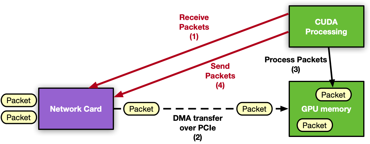
 On Aug. 8, Jensen Huang features new NVIDIA technologies and award-winning research for content creation.