
Deep learning has recently driven tremendous progress in a wide array of applications, ranging from realistic image generation and impressive retrieval systems to language models that can hold human-like conversations. While this progress is very exciting, the widespread use of deep neural network models requires caution: as guided by Google’s AI Principles, we seek to develop AI technologies responsibly by understanding and mitigating potential risks, such as the propagation and amplification of unfair biases and protecting user privacy.
Fully erasing the influence of the data requested to be deleted is challenging since, aside from simply deleting it from databases where it’s stored, it also requires erasing the influence of that data on other artifacts such as trained machine learning models. Moreover, recent research [1, 2] has shown that in some cases it may be possible to infer with high accuracy whether an example was used to train a machine learning model using membership inference attacks (MIAs). This can raise privacy concerns, as it implies that even if an individual’s data is deleted from a database, it may still be possible to infer whether that individual’s data was used to train a model.
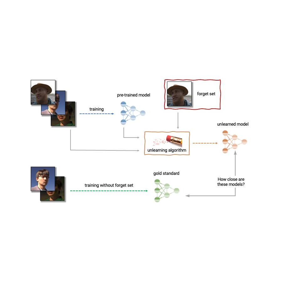
Given the above, machine unlearning is an emergent subfield of machine learning that aims to remove the influence of a specific subset of training examples — the “forget set” — from a trained model. Furthermore, an ideal unlearning algorithm would remove the influence of certain examples while maintaining other beneficial properties, such as the accuracy on the rest of the train set and generalization to held-out examples. A straightforward way to produce this unlearned model is to retrain the model on an adjusted training set that excludes the samples from the forget set. However, this is not always a viable option, as retraining deep models can be computationally expensive. An ideal unlearning algorithm would instead use the already-trained model as a starting point and efficiently make adjustments to remove the influence of the requested data.
Today we’re thrilled to announce that we’ve teamed up with a broad group of academic and industrial researchers to organize the first Machine Unlearning Challenge. The competition considers a realistic scenario in which after training, a certain subset of the training images must be forgotten to protect the privacy or rights of the individuals concerned. The competition will be hosted on Kaggle, and submissions will be automatically scored in terms of both forgetting quality and model utility. We hope that this competition will help advance the state of the art in machine unlearning and encourage the development of efficient, effective and ethical unlearning algorithms.
Machine unlearning applications
Machine unlearning has applications beyond protecting user privacy. For instance, one can use unlearning to erase inaccurate or outdated information from trained models (e.g., due to errors in labeling or changes in the environment) or remove harmful, manipulated, or outlier data.
The field of machine unlearning is related to other areas of machine learning such as differential privacy, life-long learning, and fairness. Differential privacy aims to guarantee that no particular training example has too large an influence on the trained model; a stronger goal compared to that of unlearning, which only requires erasing the influence of the designated forget set. Life-long learning research aims to design models that can learn continuously while maintaining previously-acquired skills. As work on unlearning progresses, it may also open additional ways to boost fairness in models, by correcting unfair biases or disparate treatment of members belonging to different groups (e.g., demographics, age groups, etc.).
 |
| Anatomy of unlearning. An unlearning algorithm takes as input a pre-trained model and one or more samples from the train set to unlearn (the “forget set”). From the model, forget set, and retain set, the unlearning algorithm produces an updated model. An ideal unlearning algorithm produces a model that is indistinguishable from the model trained without the forget set. |
Challenges of machine unlearning
The problem of unlearning is complex and multifaceted as it involves several conflicting objectives: forgetting the requested data, maintaining the model’s utility (e.g., accuracy on retained and held-out data), and efficiency. Because of this, existing unlearning algorithms make different trade-offs. For example, full retraining achieves successful forgetting without damaging model utility, but with poor efficiency, while adding noise to the weights achieves forgetting at the expense of utility.
Furthermore, the evaluation of forgetting algorithms in the literature has so far been highly inconsistent. While some works report the classification accuracy on the samples to unlearn, others report distance to the fully retrained model, and yet others use the error rate of membership inference attacks as a metric for forgetting quality [4, 5, 6].
We believe that the inconsistency of evaluation metrics and the lack of a standardized protocol is a serious impediment to progress in the field — we are unable to make direct comparisons between different unlearning methods in the literature. This leaves us with a myopic view of the relative merits and drawbacks of different approaches, as well as open challenges and opportunities for developing improved algorithms. To address the issue of inconsistent evaluation and to advance the state of the art in the field of machine unlearning, we’ve teamed up with a broad group of academic and industrial researchers to organize the first unlearning challenge.
Announcing the first Machine Unlearning Challenge
We are pleased to announce the first Machine Unlearning Challenge, which will be held as part of the NeurIPS 2023 Competition Track. The goal of the competition is twofold. First, by unifying and standardizing the evaluation metrics for unlearning, we hope to identify the strengths and weaknesses of different algorithms through apples-to-apples comparisons. Second, by opening this competition to everyone, we hope to foster novel solutions and shed light on open challenges and opportunities.
The competition will be hosted on Kaggle and run between mid-July 2023 and mid-September 2023. As part of the competition, today we’re announcing the availability of the starting kit. This starting kit provides a foundation for participants to build and test their unlearning models on a toy dataset.
The competition considers a realistic scenario in which an age predictor has been trained on face images, and, after training, a certain subset of the training images must be forgotten to protect the privacy or rights of the individuals concerned. For this, we will make available as part of the starting kit a dataset of synthetic faces (samples shown below) and we’ll also use several real-face datasets for evaluation of submissions. The participants are asked to submit code that takes as input the trained predictor, the forget and retain sets, and outputs the weights of a predictor that has unlearned the designated forget set. We will evaluate submissions based on both the strength of the forgetting algorithm and model utility. We will also enforce a hard cut-off that rejects unlearning algorithms that run slower than a fraction of the time it takes to retrain. A valuable outcome of this competition will be to characterize the trade-offs of different unlearning algorithms.
 |
| Excerpt images from the Face Synthetics dataset together with age annotations. The competition considers the scenario in which an age predictor has been trained on face images like the above, and, after training, a certain subset of the training images must be forgotten. |
For evaluating forgetting, we will use tools inspired by MIAs, such as LiRA. MIAs were first developed in the privacy and security literature and their goal is to infer which examples were part of the training set. Intuitively, if unlearning is successful, the unlearned model contains no traces of the forgotten examples, causing MIAs to fail: the attacker would be unable to infer that the forget set was, in fact, part of the original training set. In addition, we will also use statistical tests to quantify how different the distribution of unlearned models (produced by a particular submitted unlearning algorithm) is compared to the distribution of models retrained from scratch. For an ideal unlearning algorithm, these two will be indistinguishable.
Conclusion
Machine unlearning is a powerful tool that has the potential to address several open problems in machine learning. As research in this area continues, we hope to see new methods that are more efficient, effective, and responsible. We are thrilled to have the opportunity via this competition to spark interest in this field, and we are looking forward to sharing our insights and findings with the community.
Acknowledgements
The authors of this post are now part of Google DeepMind. We are writing this blog post on behalf of the organization team of the Unlearning Competition: Eleni Triantafillou*, Fabian Pedregosa* (*equal contribution), Meghdad Kurmanji, Kairan Zhao, Gintare Karolina Dziugaite, Peter Triantafillou, Ioannis Mitliagkas, Vincent Dumoulin, Lisheng Sun Hosoya, Peter Kairouz, Julio C. S. Jacques Junior, Jun Wan, Sergio Escalera and Isabelle Guyon.


 Debugging code is a crucial aspect of software development but can be both challenging and time-consuming. Parallel programming with thousands of threads can…
 Developers are using Universal Scene Description (OpenUSD) to push the boundaries of 3D workflows. As an ecosystem and interchange paradigm, OpenUSD models,…
 AI models are everywhere, in the form of chatbots, classification and summarization tools, image models for segmentation and detection, recommendation models,…
 Read about an innovative GPU solution that solves limitations using small biased datasets with RAPIDS cuDF.