 Join this AMA on June 28 and ask our experts how to build an AI-powered extension for NVIDIA Omniverse using ChatGPT.
Join this AMA on June 28 and ask our experts how to build an AI-powered extension for NVIDIA Omniverse using ChatGPT.
 DataBloom
Join this AMA on June 28 and ask our experts how to build an AI-powered extension for NVIDIA Omniverse using ChatGPT.
Join this AMA on June 28 and ask our experts how to build an AI-powered extension for NVIDIA Omniverse using ChatGPT.
Rendered.ai is easing AI training for developers, data scientists and others with its platform-as-a-service for synthetic data generation, or SDG. Training computer vision AI models requires massive, high-quality, diverse and unbiased datasets. These can be challenging and costly to obtain, especially with increasing demands both of and for AI. The Rendered.ai platform-as-a-service helps to solve Read article >
For industrial businesses to reach the next level of digitalization, they need to create accurate, virtual representations of their physical systems. NVIDIA is working with Hexagon, the Stockholm-based global leader in digital reality solutions combining sensor, software and autonomous technologies, to equip enterprises with the tools and solutions they need to build physically accurate, perfectly Read article >
 Apache Spark is an industry-leading platform for distributed extract, transform, and load (ETL) workloads on large-scale data. However, with the advent of deep…
Apache Spark is an industry-leading platform for distributed extract, transform, and load (ETL) workloads on large-scale data. However, with the advent of deep learning (DL), many Spark practitioners have sought to add DL models to their data processing pipelines across a variety of use cases like sales predictions, content recommendations, sentiment analysis, and fraud detection.
Yet, combining DL training and inference with large-scale data has historically been a challenge for Spark users. Most of the DL frameworks were designed for single-node environments, and their distributed training and inference APIs were often added as an after-thought.
To help solve this disconnect between the single-node DL environments and large-scale distributed environments, there are multiple third-party solutions such as Horovod-on-Spark, TensorFlowOnSpark, and SparkTorch. But, since these solutions were not natively built into Spark, users must evaluate each platform against their own needs.
With the release of Spark 3.4, users now have access to built-in APIs for both distributed model training and model inference at scale, as detailed below.
For distributed training, there is a new TorchDistributor API for PyTorch, which follows the spark-tensorflow-distributor API for TensorFlow. These simplify the migration of distributed DL model training code to Spark by taking advantage of Spark’s barrier execution mode to spawn the distributed DL cluster nodes on top of the Spark executors.
Once the DL cluster has been started by Spark, control is essentially handed off to the DL frameworks through the main_fn that was passed to the TorchDistributor API.
As shown in the following code, only minimal code changes are required to run standard distributed DL training on Spark with this new API.
from pyspark.ml.torch.distributor import TorchDistributor

def main_fn(checkpoint_dir):
    # standard distributed PyTorch code
    ...

# Set num_processes = NUM_WORKERS * NUM_GPUS_PER_WORKER
output_dist = TorchDistributor(num_processes=2, local_mode=False, use_gpu=True).run(main_fn, checkpoint_dir)
Once launched, the processes running on the executors rely on the built-in distributed training APIs of their respective DL frameworks. There should be few or no modifications required to port existing distributed training code to Spark. The processes can then communicate with each other during training and also directly access the distributed file system associated with the Spark cluster (Figure 1).
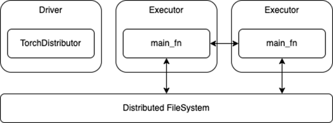
TorchDistributor APIHowever, this ease of migration also means that these APIs do not use Spark RDDs or DataFrames for data transfer. While this removes any need to translate or serialize data between Spark and the DL frameworks, it also requires that any Spark preprocessing is done and persisted to storage before launching the training job. The main training functions may also need to be adapted to read from a distributed file system instead of a local store.
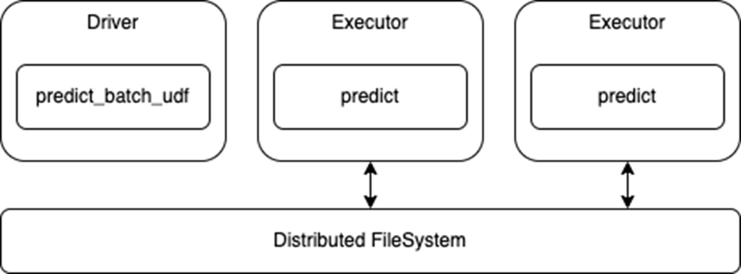
For distributed inference, there is a new predict_batch_udf API, which builds on the Spark Pandas UDF to provide a simpler interface for DL model inference. Pandas UDFs provide several advantages over row-based UDFs, including faster serialization of data through Apache Arrow and faster vectorized operations through Pandas. For more details, see Introducing Pandas UDF for PySpark.
However, while the Pandas UDF API may be a great solution for ETL use cases, it is still not ideal for DL inference use cases. First, the Pandas UDF API presents the data as a Pandas Series or DataFrame, which again is suitable for performing ETL operations like selection, sorting, math transforms, and aggregations.
Yet most DL frameworks expect either NumPy arrays or standard Python arrays as input, and these are often wrapped by custom Tensor variables. So, at a minimum, a Pandas UDF implementation needs to translate the incoming Pandas data to NumPy arrays. Unfortunately, the exact translation can vary greatly depending on the use case and dataset.
Next, the Pandas UDF API generally operates on partitions of data whose size is determined by either the original writer of the dataset or the distributed file system. As such, it can be difficult to properly batch incoming data for optimal compute.
Finally, there is still the issue of loading the DL models across the Spark executors and tasks. In a normal Spark ETL job, the workload follows a functional programming paradigm, where stateless functions can be applied against the data. However, for DL inference, the predict function typically needs to load its DL model weights from disk.
Spark has the capability to serialize variables from the driver to the executors through task serialization and broadcast variables. However, these both rely on Python pickle serialization, which may not work for all DL models. Additionally, loading and serializing very large models can be extremely costly for performance, if not done properly.
To solve these problems, the predict_batch_udf introduces standardized code for:
spark.python.worker.reuse configuration to cache models in the Spark executors.The code presented below demonstrates how this new API hides the complexity of translating DL inferencing code to Spark. The user simply defines a make_predict_fn function, using standard DL APIs, to load the model and return a predict function. Then, the predict_batch_udf function generates a standard PandasUDF, which takes care of everything else behind the scenes.
from pyspark.ml.functions import predict_batch_udf

def make_predict_fn():
    # load model from checkpoint
    import torch
    device = torch.device("cuda")
    model = Net().to(device)
    checkpoint = load_checkpoint(checkpoint_dir)
    model.load_state_dict(checkpoint['model'])

    # define predict function in terms of numpy arrays
    def predict(inputs: np.ndarray) -> np.ndarray:
        torch_inputs = torch.from_numpy(inputs).to(device)
        outputs = model(torch_inputs)
        return outputs.cpu().detach().numpy()

    return predict

# create standard PandasUDF from predict function
mnist = predict_batch_udf(make_predict_fn,
                          input_tensor_shapes=[[1,28,28]],
                          return_type=ArrayType(FloatType()),
                          batch_size=1000)

df = spark.read.parquet("/path/to/test/data")
preds = df.withColumn("preds", mnist('data')).collect()
Note that this API uses the standard Spark DataFrame for inference, so the executors will read from the distributed file system and pass that data to your predict function (Figure 2). This also means that any processing of the data can be done inline with the model prediction, as needed.
Also note that this is a data-parallel architecture, where each executor loads the model and predicts on their portions of the dataset, so the model must fit in the executor memory.
predict_batch_udf APITo try these new APIs, check out the Spark DL Training and Inference Notebook for an end-to-end example. Based on the Distributed Training E2E on Databricks Notebook from Databricks, the example notebook demonstrates:
TorchDistributor API.predict_batch_udf API for distributed inference.If you are working with common DL frameworks such as Hugging Face, PyTorch, and TensorFlow, check out the example notebooks for external frameworks. These examples demonstrate the ease of using the new predict_batch_udf API and its broad applicability.
Learn more about this API at the 2023 Data+AI Summit session, An API for Deep Learning Inferencing on Apache Spark.
 Data labeling and model training are consistently ranked as the most significant challenges teams face when building an AI/ML infrastructure. Both are essential…
Data labeling and model training are consistently ranked as the most significant challenges teams face when building an AI/ML infrastructure. Both are essential steps in the ML application development process, and if not done correctly, they can lead to inaccurate results and decreased performance. See the AI Infrastructure Ecosystem of 2022 report from the AI Infrastructure Alliance for more details.
Data labeling is essential for all forms of supervised learning, in which an entire dataset is fully labeled. It is also a key ingredient of semi-supervised learning, which combines a smaller set of labeled data with algorithms designed to automate the labeling of the rest of the dataset programmatically. Labeling is essential to computer vision, one of the most advanced and developed areas of machine learning. Despite its importance, labeling is slow because it requires scaling a distributed human labor team.
Model training is another major bottleneck in machine learning, alongside labeling. Training is slow because it involves waiting for machines to finish complex calculations. It requires teams to know about networking, distributed systems, storage, specialized processors (GPUs or TPUs), and cloud management systems (Kubernetes and Docker).
Superb AI has introduced a new way for computer vision teams to drastically decrease the time it takes to deliver high-quality training datasets. Instead of relying on human labelers for a majority of the data preparation workflow, teams can now implement a much more time- and cost-efficient pipeline with the Superb AI Suite.
NVIDIA TAO Toolkit, built on TensorFlow and PyTorch, is a low-code version of the TAO framework that accelerates the model development process by abstracting away the framework complexity. TAO Toolkit enables you to use the power of transfer learning to fine-tune NVIDIA pretrained models with your own data and optimize for inference.
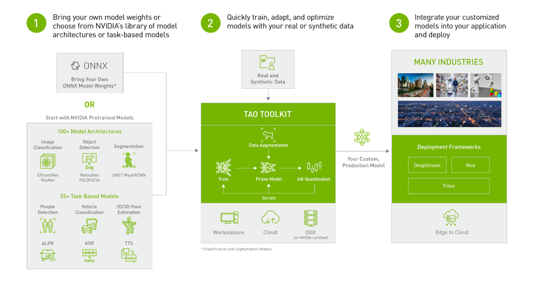
Computer vision engineers can use the Superb AI Suite and the TAO Toolkit in combination to address the challenges of data labeling and model training. More specifically, you can quickly generate labeled data in Suite and train models with TAO to perform specific computer vision tasks, whether classification, detection, or segmentation.
This post demonstrates how to use Superb AI Suite to prepare a high-quality computer vision dataset that is compatible with TAO Toolkit. It walks through the process of downloading the dataset, creating a new project on Suite, uploading data to the project through Suite SDK, using Superb AI’s Auto-Label capability to quickly label the dataset, exporting the labeled dataset, and setting up a TAO Toolkit configuration to use the data.
First, head over to superb-ai.com to create an account. Then follow the quick-start guide to install and authenticate Suite CLI. You should be able to install the latest version of spb-cli and retrieve the Suite Account Name / Access Key for authentication.
This tutorial works with the COCO dataset, a large-scale object detection, segmentation, and captioning dataset that is popular in the computer vision research community.
You can use this code snippet to download the dataset. Save it in a file called download-coco.sh and run bash download-coco.sh from the terminal. This will create a data/ directory that stores the COCO dataset.
The next step is to convert COCO to Suite SDK format to sample the five most frequent classes in the COCO validation 2017 dataset. This tutorial handles bounding box annotations only, but Suite can also handle polygons and key points.
You can use this code snippet to perform the conversion. Save it in a file called convert.py and run python convert.py from the terminal. This will create an upload-info.json file that stores information about the image name and annotations.
Creating projects through Suite SDK is a work in progress. For this tutorial, create a project on the web using the Superb AI guide for project creation. Follow the configuration presented below.
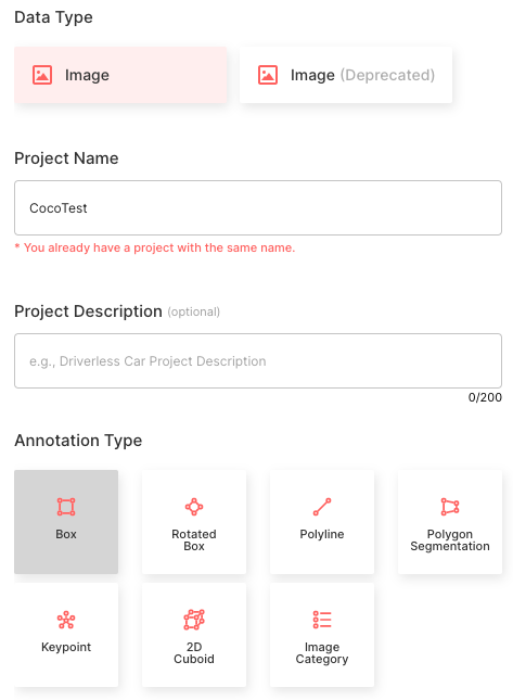
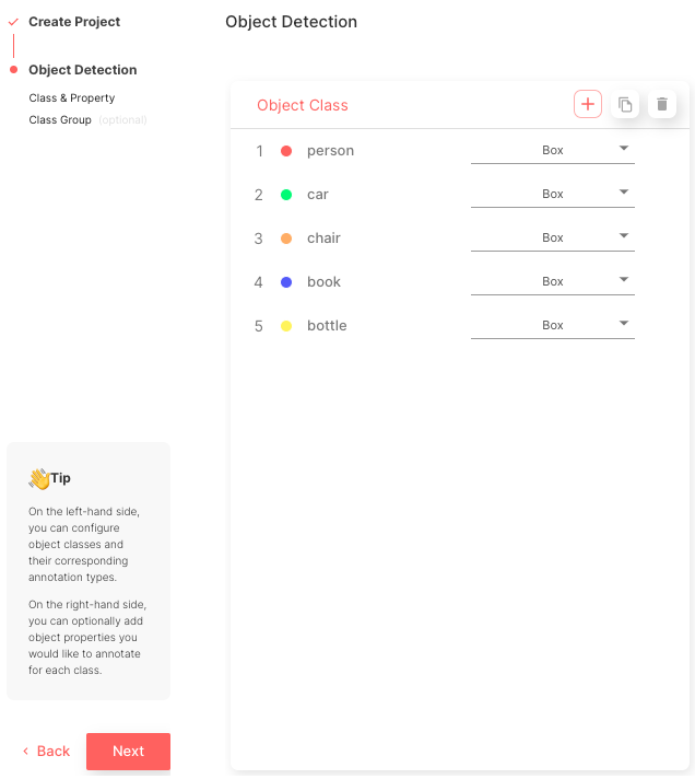
After this process is complete, you can view the main project page, as shown in Figure 5.

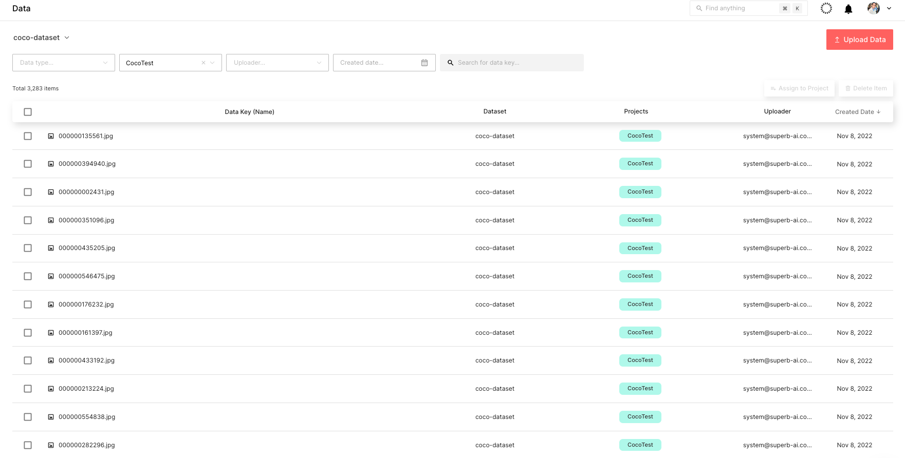
After you finish creating the project, start uploading the data. You can use this code snippet to upload the data. Save it in a file called upload.py and run python upload.py --project CocoTest --dataset coco-dataset in the terminal.
That means CocoTest is the project name and coco-dataset is the dataset name. This will kickstart the uploading process, which can take several hours to complete, depending on the processing power of the device.
You can check the uploaded dataset through the Suite web page in real time, as shown in Figure 6.
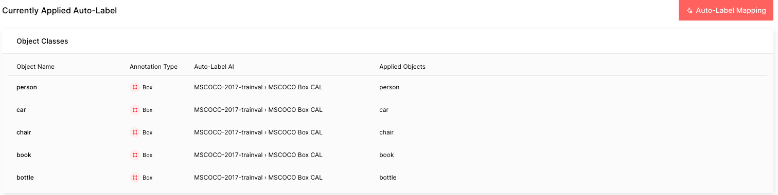
The next step is to label the COCO dataset. To do so quickly, use Suite’s powerful automated labeling capabilities. More specifically, Auto-Label and Custom Auto-Label are both powerful tools that can boost labeling efficiency by automatically detecting objects and labeling them.
Auto-Label is a pretrained model developed by Superb AI that detects and labels 100+ common objects, whereas Custom Auto-Label is a model trained using your own data that detects and labels niche objects.
The COCO data in this tutorial is composed of five common objects that Auto-Label is capable of labeling. Follow the guide to configure Auto-Label. The important thing to remember is that you would want to choose the MSCOCO Box CAL as the Auto-Label AI and map the object names with the respective applied objects. It can take about an hour to process all 3,283 labels in the COCO dataset.
After the Auto-Label finishes running, you will see the difficulty of each automated labeling task: red is difficult, yellow is moderate, and green is easy. The higher the difficulty is, the more likely that the Auto-Label incorrectly labeled that image.
This level of difficulty, or estimated uncertainty, is calculated based on factors such as small object size, bad lighting conditions, complex scenes, and so on. In a real-world situation, you can easily sort and filter labels by difficulty in order to prioritize going over labels with a higher chance of errors.
After obtaining the labeled dataset, export and download the labels. There is more to a label than just the annotation information. In order to fully use a label for training ML models, you must know additional information, such as the project configuration and meta-information about the raw data. To download all this information along with the annotation files, first request an export so that the Suite system can create a zip file for download. Follow the guide to export and download labels from the Suite.
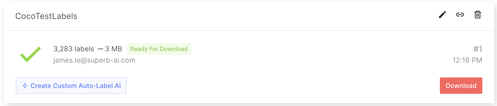
When you export labels, a compressed zip file will be created for you to download. The export result folder will contain general information regarding the project as a whole, annotation information for each label, and the metadata for each data asset. For more details, see the Export Result Format documentation.
Next, create a script to convert your labeled data to a format that can be input to TAO Toolkit, such as the COCO format. Note that because this tutorial uses the COCO dataset, the data is already in the COCO format. For instance, you can find the JSON file below of a random exported label:
{
   "objects": [
       {
           "id": "7e9fe8ee-50c7-4d4f-9e2c-145d894a8a26",
           "class_id": "7b8205ef-b251-450c-b628-e6b9cac1a457",
           "class_name": "person",
           "annotation_type": "box",
           "annotation": {
               "multiple": false,
               "coord": {
                   "x": 275.47,
                   "y": 49.27,
                   "width": 86.39999999999998,
                   "height": 102.25
               },
               "meta": {},
               "difficulty": 0,
               "uncertainty": 0.0045
           },
           "properties": []
       },
       {
           "id": "70257635-801f-4cad-856a-ef0fdbfdf613",
           "class_id": "7b8205ef-b251-450c-b628-e6b9cac1a457",
           "class_name": "person",
           "annotation_type": "box",
           "annotation": {
               "multiple": false,
               "coord": {
                   "x": 155.64,
                   "y": 40.61,
                   "width": 98.34,
                   "height": 113.05
               },
               "meta": {},
               "difficulty": 0,
               "uncertainty": 0.0127
           },
           "properties": []
       }
   ],
   "categories": {
       "properties": []
   },
   "difficulty": 1
}Next, pull the COCO data from Suite into model development by using SuiteDataset. SuiteDataset makes an exported dataset within the Suite accessible through the PyTorch data pipeline. The code snippet shown below instantiates the SuiteDataset object class for your training set.
class SuiteDataset(Dataset):
   """
   Instantiate the SuiteDataset object class for training set
   """

   def __init__(
           self,
           team_name: str,
           access_key: str,
           project_name: str,
           export_name: str,
           train: bool,
           caching_image: bool = True,
           transforms: Optional[List[Callable]] = None,
           category_names: Optional[List[str]] = None,
   ):
       """Function to initialize the object class"""
       super().__init__()

       # Get project setting and export information through the SDK
       # Initialize the Python Client
       client = spb.sdk.Client(team_name=team_name, access_key=access_key, project_name=project_name)
       # Use get_export
       export_info = call_with_retry(client.get_export, name=export_name)
       # Download the export compressed file through download_url in Export
       export_data = call_with_retry(urlopen, export_info.download_url).read()

       # Load the export compressed file into memory
       with ZipFile(BytesIO(export_data), 'r') as export:
           label_files = [f for f in export.namelist() if f.startswith('labels/')]
           label_interface = json.loads(export.open('project.json', 'r').read())
           category_infos = label_interface.get('object_detection', {}).get('object_classes', [])

       cache_dir = None
       if caching_image:
           cache_dir = f'/tmp/{team_name}/{project_name}'
           os.makedirs(cache_dir, exist_ok=True)

       self.client = client
       self.export_data = export_data
       self.categories = [
           {'id': i + 1, 'name': cat['name'], 'type': cat['annotation_type']}
           for i, cat in enumerate(category_infos)
       ]
       self.category_id_map = {cat['id']: i + 1 for i, cat in enumerate(category_infos)}
       self.transforms = build_transforms(train, self.categories, transforms, category_names)
       self.cache_dir = cache_dir

       # Convert label_files to numpy array and use
       self.label_files = np.array(label_files).astype(np.string_)

   def __len__(self):
       """Function to return the number of label files"""
       return len(self.label_files)

   def __getitem__(self, idx):
       """Function to get an item"""
       idx = idx if idx >= 0 else len(self) + idx
       if idx = len(self):
           raise IndexError(f'index out of range')

       image_id = idx + 1
       label_file = self.label_files[idx].decode('ascii')

       # Load label information corresponding to idx from the export compressed file into memory
       with ZipFile(BytesIO(self.export_data), 'r') as export:
           label = load_label(export, label_file, self.category_id_map, image_id)

       # Download the image through the Suite sdk based on label_id
       try:
           image = load_image(self.client, label['label_id'], self.cache_dir)
       # Download data in real time using get_data from Suite sdk
       except Exception as e:
           print(f'Failed to load the {idx}-th image due to {repr(e)}, getting {idx + 1}-th data instead')
           return self.__getitem__(idx + 1)

       target = {
           'image_id': image_id,
           'label_id': label['label_id'],
           'annotations': label['annotations'],
       }

       if self.transforms is not None:
           image, target = self.transforms(image, target)
       return image, target
Handle the test set in a similar fashion. The code snippet below instantiates the SuiteCocoDataset object class for the test set by wrapping SuiteDataset to make it compatible with the Torchvision COCOEvaluator.
class SuiteCocoDataset(C.CocoDetection):
   """
   Instantiate the SuiteCocoDataset object class for test set
   (by wrapping SuiteDataset to make compatible with torchvision's official COCOEvaluator)
   """

   def __init__(
           self,
           team_name: str,
           access_key: str,
           project_name: str,
           export_name: str,
           train: bool,
           caching_image: bool = True,
           transforms: Optional[List[Callable]] = None,
           category_names: Optional[List[str]] = None,
           num_init_workers: int = 20,
   ):
       """Function to initialize the object class"""
       super().__init__(img_folder='', ann_file=None, transforms=None)

       # Call the SuiteDataset class
       dataset = SuiteDataset(
           team_name, access_key, project_name, export_name,
           train=False, transforms=[],
           caching_image=caching_image, category_names=category_names,
       )
       self.client = dataset.client
       self.cache_dir = dataset.cache_dir

       self.coco = build_coco_dataset(dataset, num_init_workers)
       self.ids = list(sorted(self.coco.imgs.keys()))
       self._transforms = build_transforms(train, dataset.categories, transforms, category_names)

   def _load_image(self, id: int):
       """Function to load an image"""
       label_id = self.coco.loadImgs(id)[0]['label_id']
       image = load_image(self.client, label_id, self.cache_dir)
       return image

   def __getitem__(self, idx):
       """Function to get an item"""
       try:
           return super().__getitem__(idx)
       except Exception as e:
           print(f'Failed to load the {idx}-th image due to {repr(e)}, getting {idx + 1}-th data instead')
           return self.__getitem__(idx + 1)
SuiteDataset and SuiteCocoDataset can then be used for your training code. The code snippet below illustrates how to use them. During model development, train with train_loader and evaluate with test_loader.
train_dataset = SuiteDataset(
   team_name=args.team_name,
   access_key=args.access_key,
   project_name=args.project_name,
   export_name=args.train_export_name,
   caching_image=args.caching_image,
   train=True,
)
test_dataset = SuiteCocoDataset(
   team_name=args.team_name,
   access_key=args.access_key,
   project_name=args.project_name,
   export_name=args.test_export_name,
   caching_image=args.caching_image,
   train=False,
   num_init_workers=args.workers,
)

train_loader = DataLoader(
   train_dataset, num_workers=args.workers,
   batch_sampler=G.GroupedBatchSampler(
       RandomSampler(train_dataset),
       G.create_aspect_ratio_groups(train_dataset, k=3),
       args.batch_size,
   ),
   collate_fn=collate_fn,
)
test_loader = DataLoader(
   test_dataset, num_workers=args.workers,
   sampler=SequentialSampler(test_dataset), batch_size=1,
   collate_fn=collate_fn,
)Your data annotated with Suite can now be used to train your object detection model. TAO Toolkit enables you to train, fine-tune, prune, and export highly optimized and accurate computer vision models for deployment by adapting popular network architectures and backbones to your data. For this tutorial, you can choose YOLO v4, an object detection model included in TAO.
First, download the notebook samples from TAO Toolkit Quick Start.
pip3 install nvidia-tao
wget --content-disposition https://api.ngc.nvidia.com/v2/resources/nvidia/tao/tao-getting-started/versions/4.0.1/zip -O getting_started_v4.0.1.zip


$ unzip -u getting_started_v4.0.1.zip  -d ./getting_started_v4.0.1 && rm -rf getting_started_v4.0.1.zip && cd ./getting_started_v4.0.1
Next, start the notebook using the code below:
$ jupyter notebook --ip 0.0.0.0 --port 8888 --allow-rootOpen your Internet browser on localhost and navigate to the URL:
http://0.0.0.0:8888To create a YOLOv4 model, open notebooks/tao_launcher_starter_kit/yolo_v4/yolo_v4.ipynb and follow the notebook instructions to train the model.
Based on the results, fine-tune the model until it achieves your metric goals. If desired, you can create your own active learning loop at this stage. In a real-world scenario, query samples of failed predictions, assign human labelers to annotate this new batch of sample data, and supplement your model with newly labeled training data. Superb AI Suite can further assist you with data collection and annotation in subsequent rounds of model development as you iteratively improve your model performance.
With the recently released TAO Toolkit 4.0, it is even easier to get started and create high-accuracy models without any AI expertise. Automatically fine-tune your hyperparameters with AutoML, experience turnkey deployment of TAO Toolkit into various cloud services, integrate TAO Toolkit with third-party MLOPs services, and explore new transformer-based vision models (CitySemSegformer, Peoplenet Transformer).
Data labeling in computer vision can present many unique challenges. The process can be difficult and expensive due to the amount of data that needs labeling. In addition, the process can be subjective, which makes it challenging to achieve consistently high-quality labeled outputs across a large dataset.
Model training can be challenging as well, as many algorithms and hyperparameters require tuning and optimization. This process requires a deep understanding of the data and the model, and significant experimentation to achieve the best results. Additionally, computer vision models tend to require large computing power to train, making it difficult to do so on a limited budget and timeline.
Superb AI Suite enables you to collect and label high-quality computer vision datasets. With NVIDIA TAO Toolkit, you can optimize pretrained computer vision models. Using both together significantly accelerates your computer vision application development times without sacrificing quality.
Want more information? Check out:
Superb AI provides a training data platform that makes building, managing, and curating computer vision datasets faster and easier than ever before. Specializing in adaptable automation models for labeling and quality assurance, our solutions help companies drastically reduce the time and cost of building data pipelines for computer vision models. Launched in 2018 by researchers and engineers with decades of experience in computer vision and deep learning (including 25+ publications, 7,300+ citations, and 100+ patents), our vision is to empower companies at all stages to develop computer vision applications faster than ever before.
Superb AI is also a proud collaborator with NVIDIA through the NVIDIA Inception Program for Startups. This program helps nurture the development of the world’s cutting-edge startups, providing them with access to NVIDIA technologies and experts, opportunities to connect with venture capitalists, and comarketing support to heighten their visibility.
 Some years ago, Jensen Huang, founder and CEO of NVIDIA, hand-delivered the world’s first NVIDIA DGX AI system to OpenAI. Fast forward to the present and…
Some years ago, Jensen Huang, founder and CEO of NVIDIA, hand-delivered the world’s first NVIDIA DGX AI system to OpenAI. Fast forward to the present and OpenAI’s ChatGPT has taken the world by storm, highlighting the benefits and capabilities of artificial intelligence (AI) and how it can be applied in every industry and business, small or enterprise.
Now, have you ever stopped to think about the technologies and infrastructure that it takes to host and support ChatGPT?
In this video, Mark Russinovich, Microsoft Azure CTO, explains the technology stack behind their purpose-built AI supercomputer infrastructure. It was developed by NVIDIA and Microsoft Azure, in collaboration with OpenAI, to host ChatGPT and other large language models (LLMs) at any scale.
When training AI models with hundreds of billions of parameters, an efficient data center infrastructure is key: from increasing throughput and minimizing server failures to leveraging multi-GPU clusters for compute-intensive workloads.
For more information about optimizing your data center infrastructure to reliably deploy large models at scale, see the following resources:
Kirk Kaiser grew up a fan of the video game Paperboy, where players act as cyclists delivering newspapers while encountering various obstacles, like ramps that appear in the middle of the street. This was the inspiration behind the software developer’s latest project using the NVIDIA Jetson platform for edge AI and robotics — a self-driving Read article >
In the last few years, text-to-image generation research has seen an explosion of breakthroughs (notably, Imagen, Parti, DALL-E 2, etc.) that have naturally permeated into related topics. In particular, text-guided image editing (TGIE) is a practical task that involves editing generated and photographed visuals rather than completely redoing them. Quick, automated, and controllable editing is a convenient solution when recreating visuals would be time-consuming or infeasible (e.g., tweaking objects in vacation photos or perfecting fine-grained details on a cute pup generated from scratch). Further, TGIE represents a substantial opportunity to improve training of foundational models themselves. Multimodal models require diverse data to train properly, and TGIE editing can enable the generation and recombination of high-quality and scalable synthetic data that, perhaps most importantly, can provide methods to optimize the distribution of training data along any given axis.
In “Imagen Editor and EditBench: Advancing and Evaluating Text-Guided Image Inpainting”, to be presented at CVPR 2023, we introduce Imagen Editor, a state-of-the-art solution for the task of masked inpainting — i.e., when a user provides text instructions alongside an overlay or “mask” (usually generated within a drawing-type interface) indicating the area of the image they would like to modify. We also introduce EditBench, a method that gauges the quality of image editing models. EditBench goes beyond the commonly used coarse-grained “does this image match this text” methods, and drills down to various types of attributes, objects, and scenes for a more fine-grained understanding of model performance. In particular, it puts strong emphasis on the faithfulness of image-text alignment without losing sight of image quality.
 |
| Given an image, a user-defined mask, and a text prompt, Imagen Editor makes localized edits to the designated areas. The model meaningfully incorporates the user’s intent and performs photorealistic edits. |
Imagen Editor is a diffusion-based model fine-tuned on Imagen for editing. It targets improved representations of linguistic inputs, fine-grained control and high-fidelity outputs. Imagen Editor takes three inputs from the user: 1) the image to be edited, 2) a binary mask to specify the edit region, and 3) a text prompt — all three inputs guide the output samples.
Imagen Editor depends on three core techniques for high-quality text-guided image inpainting. First, unlike prior inpainting models (e.g., Palette, Context Attention, Gated Convolution) that apply random box and stroke masks, Imagen Editor employs an object detector masking policy with an object detector module that produces object masks during training. Object masks are based on detected objects rather than random patches and allow for more principled alignment between edit text prompts and masked regions. Empirically, the method helps the model stave off the prevalent issue of the text prompt being ignored when masked regions are small or only partially cover an object (e.g., CogView2).
 |
| Random masks (left) frequently capture background or intersect object boundaries, defining regions that can be plausibly inpainted just from image context alone. Object masks (right) are harder to inpaint from image context alone, encouraging models to rely more on text inputs during training. |
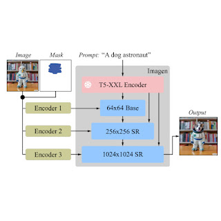
Next, during training and inference, Imagen Editor enhances high resolution editing by conditioning on full resolution (1024×1024 in this work), channel-wise concatenation of the input image and the mask (similar to SR3, Palette, and GLIDE). For the base diffusion 64×64 model and the 64×64→256×256 super-resolution models, we apply a parameterized downsampling convolution (e.g., convolution with a stride), which we empirically find to be critical for high fidelity.
 |
| Imagen is fine-tuned for image editing. All of the diffusion models, i.e., the base model and super-resolution (SR) models, are conditioned on high-resolution 1024×1024 image and mask inputs. To this end, new convolutional image encoders are introduced. |
Finally, at inference we apply classifier-free guidance (CFG) to bias samples to a particular conditioning, in this case, text prompts. CFG interpolates between the text-conditioned and unconditioned model predictions to ensure strong alignment between the generated image and the input text prompt for text-guided image inpainting. We follow Imagen Video and use high guidance weights with guidance oscillation (a guidance schedule that oscillates within a value range of guidance weights). In the base model (the stage-1 64x diffusion), where ensuring strong alignment with text is most critical, we use a guidance weight schedule that oscillates between 1 and 30. We observe that high guidance weights combined with oscillating guidance result in the best trade-off between sample fidelity and text-image alignment.
The EditBench dataset for text-guided image inpainting evaluation contains 240 images, with 120 generated and 120 natural images. Generated images are synthesized by Parti and natural images are drawn from the Visual Genome and Open Images datasets. EditBench captures a wide variety of language, image types, and levels of text prompt specificity (i.e., simple, rich, and full captions). Each example consists of (1) a masked input image, (2) an input text prompt, and (3) a high-quality output image used as reference for automatic metrics. To provide insight into the relative strengths and weaknesses of different models, EditBench prompts are designed to test fine-grained details along three categories: (1) attributes (e.g., material, color, shape, size, count); (2) object types (e.g., common, rare, text rendering); and (3) scenes (e.g., indoor, outdoor, realistic, or paintings). To understand how different specifications of prompts affect model performance, we provide three text prompt types: a single-attribute (Mask Simple) or a multi-attribute description of the masked object (Mask Rich) – or an entire image description (Full Image). Mask Rich, especially, probes the models’ ability to handle complex attribute binding and inclusion.
 |
| The full image is used as a reference for successful inpainting. The mask covers the target object with a free-form, non-hinting shape. We evaluate Mask Simple, Mask Rich and Full Image prompts, consistent with conventional text-to-image models. |
Due to the intrinsic weaknesses in existing automatic evaluation metrics (CLIPScore and CLIP-R-Precision) for TGIE, we hold human evaluation as the gold standard for EditBench. In the section below, we demonstrate how EditBench is applied to model evaluation.
We evaluate the Imagen Editor model — with object masking (IM) and with random masking (IM-RM) — against comparable models, Stable Diffusion (SD) and DALL-E 2 (DL2). Imagen Editor outperforms these models by substantial margins across all EditBench evaluation categories.
For Full Image prompts, single-image human evaluation provides binary answers to confirm if the image matches the caption. For Mask Simple prompts, single-image human evaluation confirms if the object and attribute are properly rendered, and bound correctly (e.g., for a red cat, a white cat on a red table would be an incorrect binding). Side-by-side human evaluation uses Mask Rich prompts only for side-by-side comparisons between IM and each of the other three models (IM-RM, DL2, and SD), and indicates which image matches with the caption better for text-image alignment, and which image is most realistic.
 |
| Human evaluation. Full Image prompts elicit annotators’ overall impression of text-image alignment; Mask Simple and Mask Rich check for the correct inclusion of particular attributes, objects and attribute binding. |
For single-image human evaluation, IM receives the highest ratings across-the-board (10–13% higher than the 2nd-highest performing model). For the rest, the performance order is IM-RM > DL2 > SD (with 3–6% difference) except for with Mask Simple, where IM-RM falls 4-8% behind. As relatively more semantic content is involved in Full and Mask Rich, we conjecture IM-RM and IM are benefited by the higher performing T5 XXL text encoder.
 |
| Single-image human evaluations of text-guided image inpainting on EditBench by prompt type. For Mask Simple and Mask Rich prompts, text-image alignment is correct if the edited image accurately includes every attribute and object specified in the prompt, including the correct attribute binding. Note that due to different evaluation designs, Full vs. Mask-only prompts, results are less directly comparable. |
EditBench focuses on fine-grained annotation, so we evaluate models for object and attribute types. For object types, IM leads in all categories, performing 10–11% better than the 2nd-highest performing model in common, rare, and text-rendering.
 |
| Single-image human evaluations on EditBench Mask Simple by object type. As a cohort, models are better at object rendering than text-rendering. |
For attribute types, IM is rated much higher (13–16%) than the 2nd highest performing model, except for in count, where DL2 is merely 1% behind.
 |
| Single-image human evaluations on EditBench Mask Simple by attribute type. Object masking improves adherence to prompt attributes across-the-board (IM vs. IM-RM). |
Side-by-side compared with other models one-vs-one, IM leads in text alignment with a substantial margin, being preferred by annotators compared to SD, DL2, and IM-RM.
 |
| Side-by-side human evaluation of image realism & text-image alignment on EditBench Mask Rich prompts. For text-image alignment, Imagen Editor is preferred in all comparisons. |
Finally, we illustrate a representative side-by-side comparative for all the models. See the paper for more examples.
 |
| Example model outputs for Mask Simple vs. Mask Rich prompts. Object masking improves Imagen Editor’s fine-grained adherence to the prompt compared to the same model trained with random masking. |
We presented Imagen Editor and EditBench, making significant advancements in text-guided image inpainting and the evaluation thereof. Imagen Editor is a text-guided image inpainting fine-tuned from Imagen. EditBench is a comprehensive systematic benchmark for text-guided image inpainting, evaluating performance across multiple dimensions: attributes, objects, and scenes. Note that due to concerns in relation to responsible AI, we are not releasing Imagen Editor to the public. EditBench on the other hand is released in full for the benefit of the research community.
Thanks to Gunjan Baid, Nicole Brichtova, Sara Mahdavi, Kathy Meier-Hellstern, Zarana Parekh, Anusha Ramesh, Tris Warkentin, Austin Waters, and Vijay Vasudevan for their generous support. We give thanks to Igor Karpov, Isabel Kraus-Liang, Raghava Ram Pamidigantam, Mahesh Maddinala, and all the anonymous human annotators for their coordination to complete the human evaluation tasks. We are grateful to Huiwen Chang, Austin Tarango, and Douglas Eck for providing paper feedback. Thanks to Erica Moreira and Victor Gomes for help with resource coordination. Finally, thanks to the authors of DALL-E 2 for giving us permission to use their model outputs for research purposes.
When meteor showers occur every few months, viewers get to watch a dazzling scene of shooting stars and light streaks scattering across the night sky. Normally, meteors are just small pieces of rock and dust from space that quickly burn up upon entering Earth’s atmosphere. But the story would take a darker turn if a Read article >
 Reconstructing a smooth surface from a point cloud is a fundamental step in creating digital twins of real-world objects and scenes. Algorithms for surface…
Reconstructing a smooth surface from a point cloud is a fundamental step in creating digital twins of real-world objects and scenes. Algorithms for surface reconstruction appear in various applications, such as industrial simulation, video game development, architectural design, medical imaging, and robotics.
Neural Kernel Surface Reconstruction (NKSR) is the new NVIDIA algorithm for reconstructing high-fidelity surfaces from large point clouds. NKSR can process millions of points in seconds and achieves state-of-the-art quality on a wide range of benchmarks. NKSR is an excellent substitute for traditional Poisson Surface Reconstruction, providing greater detail and faster runtimes.
NKSR leverages a novel 3D deep learning approach called Neural Kernel Fields to achieve high-quality reconstruction. First introduced in 2022 by the NVIDIA Toronto AI Lab, Neural Kernel Fields predict a data-dependent set of basis functions used to solve the closed-form surface reconstruction problem. This new approach enables unprecedented generalization (for training on objects and reconstructing scenes) and multimodal training on scenes and objects at different scales. For more technical details about the method, visit the NKSR project page.
Alongside the code release, we are excited to introduce the kitchen sink model, a comprehensive model trained on datasets of varying scales. By incorporating object-level and scene-level data, we have ensured the model’s versatility across different scenarios. To demonstrate its effectiveness, we have successfully applied the kitchen sink model to diverse datasets.
Figure 2 shows a room-level reconstruction result using a sparse input point cloud. Our method outperforms other baselines by generating smooth and accurate geometry.
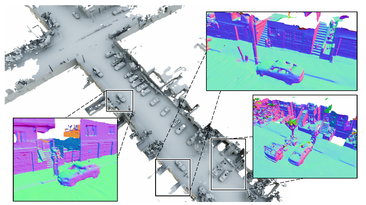
Figure 3 showcases the application of our method on a race track, and Figure 4 shows a neighborhood scene. These scenes were captured using an autonomous vehicle equipped with a lidar sensor. Both scenes span several kilometers in length, and we were able to efficiently process them on a GPU.
NKSR is easily accessible through pip, with PyTorch being a key dependency. This integration enables the direct installation of the package, ensuring a streamlined setup process.
Use the following installation command:
pip install nksr -f https://nksr.s3.ap-northeast-1.amazonaws.com/whl/torch-2.0.0%2Bcu118.htmlThe core computing operations of NKSR are accelerated using GPU, which results in high-speed processing and efficient performance. When deploying NKSR, it is necessary to define the positions and normals of your input point cloud. Alternatively, you can input the positions of the sensors capturing these points.
The code snippet below demonstrates how easy it is to use NKSR:
import nksr
import torch

device = torch.device("cuda:0")
reconstructor = nksr.Reconstructor(device)

# Note that input_xyz and input_normal are torch tensors of shape [N, 3] and [N, 3] respectively.
field = reconstructor.reconstruct(input_xyz, input_normal)
# input_color is also a tensor of shape [N, 3]
field.set_texture_field(nksr.fields.PCNNField(input_xyz, input_color))
# Increase the dual mesh's resolution.
mesh = field.extract_dual_mesh(mise_iter=2)

# Visualizing
from pycg import vis
vis.show_3d([vis.mesh(mesh.v, mesh.f, color=mesh.c)])
The culmination of this process is a triangulated mesh, which you can save directly or visualize based on your specific needs.
If the default configuration (kitchen sink model) does not adequately meet your requirements, the training code is provided. This additional resource offers the flexibility to train a custom model or to integrate NKSR into your existing pipeline. Our commitment to customization and usability ensures that NKSR can be adapted to various applications and scenarios.
NVIDIA Neural Kernel Surface Reconstruction presents a novel and cutting-edge approach to extract high-quality 3D surfaces from sparse point clouds. By employing a sparse Neural Kernel Field approach, the NKSR kitchen sink model can generalize to arbitrary inputs at any scale from a fixed training set of shapes. NKSR is fully open source and comes with training code and the pretrained kitchen sink model, which you can install directly with pip. You can further fine-tune NKSR to your specific datasets and problem domains, to enable even higher reconstruction quality in specialized applications.
We want to see what you can do with NKSR. Demonstrate your most impressive reconstruction results and captivating visualizations using NKSR. Then enter the NVIDIA NKSR Sweepstakes by September 8, 2023 for your chance to win a GeForce RTX 3090 Ti.