
 A growing number of network applications need to exercise GPU real-time packet processing in order to implement high data rate solutions: data filtering, data…
A growing number of network applications need to exercise GPU real-time packet processing in order to implement high data rate solutions: data filtering, data placement, network analysis, sensors’ signal processing, and more.
One primary motivation is the high degree of parallelism that the GPU can enable to process in parallel multiple packets while offering scalability and programmability.
For an overview of the basic concepts of these techniques and an initial solution based on the DPDK gpudev library, see Boosting Inline Packet Processing Using DPDK and GPUdev with GPUs.
This post explains how the new NVIDIA DOCA GPUNetIO Library can overcome some of the limitations found in the previous DPDK solution, moving a step closer to GPU-centric packet processing applications.
Introduction
Real-time GPU processing of network packets is a technique useful to several different application domains, including signal processing, network security, information gathering, and input reconstruction. The goal of these applications is to realize an inline packet processing pipeline to receive packets in GPU memory (without staging copies through CPU memory); process them in parallel with one or more CUDA kernels; and then run inference, evaluate, or send over the network the result of the calculation.
Typically, in this pipeline, the CPU is the intermediary because it has to synchronize network card (NIC) receive activity with the GPU processing. This wakes up the CUDA kernel as soon as new packets have been received in GPU memory. Similar considerations can be applied to the send side of the pipeline.
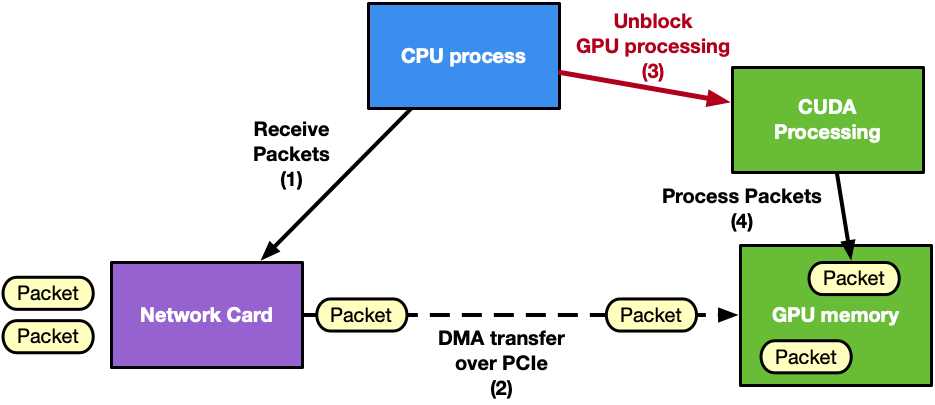
The Data Plane Development Kit (DPDK) framework introduced the gpudev library to provide a solution for this kind of application: receive or send using GPU memory (GPUDirect RDMA technology) in combination with low-latency CPU synchronization. For more information about different approaches to coordinating CPU and GPU activity, see Boosting Inline Packet Processing Using DPDK and GPUdev with GPUs.
GPU-initiated communications
Looking at Figure 1, it is clear that the CPU is the main bottleneck. It has too many responsibilities in synchronizing NIC and GPU tasks and managing multiple network queues. As an example, consider an application with many receive queues and an incoming traffic of 100 Gbps. A CPU-centric solution would have:
- CPU invoking the network function on each receive queue to receive packets in GPU memory using one or multiple CPU cores
- CPU collecting packets’ info (packets addresses, number)
- CPU notifying the GPU about new received packets
- GPU processing the packets
This CPU-centric approach is:
- Resource consuming: To deal with high-rate network throughput (100 Gbps or more) the application may need to dedicate an entire CPU physical core to receive (and/or send) packets
- Not scalable: In order to receive (or send) in parallel with different queues, the application may need to use multiple CPU cores even on systems where the total number of CPU cores may be limited to a low number (depending on the platform)
- Platform dependent: The same application on a low-power CPU will decrease the performance
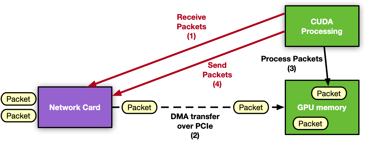
The next natural step for GPU inline packet processing applications is to remove the CPU from the critical path. Moving to a GPU-centric solution, the GPU can directly interact with the NIC to receive packets so the processing can start as soon as packets arrive in GPU memory. The same considerations can be applied to the send operation.
The capability of a GPU to control the NIC activity from a CUDA kernel is called GPU-initiated communications. Assuming the use of an NVIDIA GPU and an NVIDIA NIC, it is possible to expose the NIC registers to the direct access of the GPU. In this way, a CUDA kernel can directly configure and update these registers to orchestrate a send or a receive network operation without the intervention of the CPU.
DPDK is, by definition, a CPU framework. To enable GPU-initiated communications, it would be necessary to move the whole control path on the GPU, which is not applicable. For this reason, this feature is enabled by creating a new NVIDIA DOCA library.
NVIDIA DOCA GPUNetIO Library
NVIDIA DOCA SDK is the new NVIDIA framework composed of drivers, libraries, tools, documentation, and example applications. These resources are needed to leverage your application with the network, security, and computation features the NVIDIA hardware can expose on host systems and DPU.
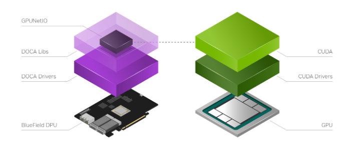
NVIDIA DOCA GPUNetIO is a new library developed on top of the NVIDIA DOCA 1.5 release to introduce the notion of a GPU device in the DOCA ecosystem (Figure 3). To facilitate the creation of a DOCA GPU-centric real-time packet processing application, DOCA GPUNetIO combines GPUDirect RDMA for data-path acceleration, smart GPU memory management, low-latency message passing techniques between CPU and GPU (through GDRCopy features) and GPU-initiated communications.
This enables a CUDA kernel to directly control an NVIDIA ConnectX network card. To maximize the performance, DOCA GPUNetIO Library must be used on platforms considered GPUDirect-friendly, where the GPU and the network card are directly connected through a dedicated PCIe bridge. The DPU converged card is an example but the same topology can be realized on host systems as well.
DOCA GPUNetIO targets are GPU packet processing network applications using the Ethernet protocol to exchange packets in a network. With these applications, there is no need for a pre synchronization phase across peers through an OOB mechanism, as for RDMA-based applications. There is also no need to assume other peers will use DOCA GPUNetIO to communicate and no need to be topology-aware. In future releases, the RDMA option will be enabled to cover more use-cases.
DOCA GPUNetIO features enabled in the current release are:
- GPU-initiated communications: A CUDA kernel can invoke the CUDA device functions in the DOCA GPUNetIO Library to instruct the network card to send or receive packets
- Accurate Send Scheduling: With GPU-initiated communications, it is possible to schedule packets’ transmission in the future according to some user-provided timestamp
- GPUDirect RDMA: Receive or send packets in contiguous fixed-size GPU memory strides without CPU memory staging copies
- Semaphores: Provide a standardized low-latency message passing protocol between CPU and GPU or between different GPU CUDA kernels
- CPU direct access to GPU memory: CPU can modify a GPU memory buffers without using CUDA memory API
As shown in Figure 4, the typical DOCA GPUNetIO application steps are:
- Initial configuration phase on CPU
- Use DOCA to identify and initialize a GPU device and a network device
- Use DOCA GPUNetIO to create receive or send queues manageable from a CUDA kernel
- Use DOCA Flow to determine which type of packet should land in each receive queue (for example, subset of IP addresses, TCP or UDP protocol, and so on)
- Launch one or more CUDA kernels (to execute packet processing/filtering/analysis)
- Runtime control and data path on GPU within CUDA kernel
- Use DOCA GPUNetIO CUDA device functions to send or receive packets
- Use DOCA GPUNetIO CUDA device functions to interact with the semaphores to synchronize the work with other CUDA kernels or with the CPU
The following sections present an overview of possible GPU packet processing pipeline application layouts combining DOCA GPUNetIO building blocks.
CPU receive and GPU process
This first example is CPU-centric and does not use the GPU-initiated communication capability. It can be considered as the baseline for the following sections. The CPU creates receive queues manageable from the CPU itself to receive packets in GPU memory and assign flow steering rules to each queue.
At runtime, the CPU receives packets in GPU memory. It notifies one or multiple CUDA kernels, through the DOCA GPUNetIO semaphores, of the arrival of a new set of packets per queue, providing information like GPU memory address and number of packets. On the GPU, the CUDA kernel, polling on the semaphore, detects the update and begins to process the packets.
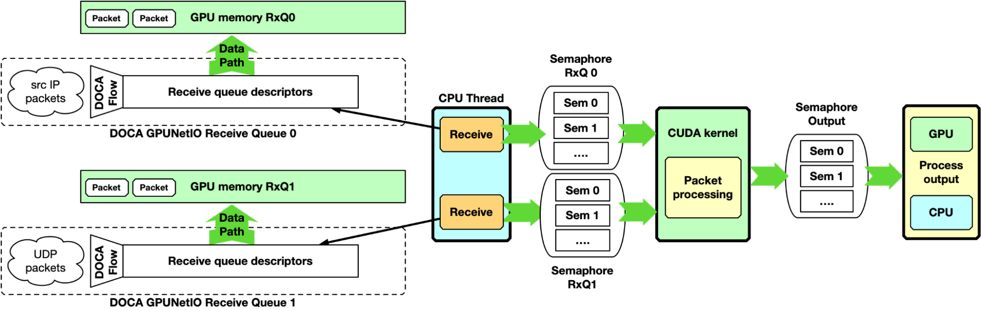
Here, the DOCA GPUNetIO semaphore has a functionality similar to the DPDK gpudev communication list, enabling a low-latency communication mechanism between the CPU receiving packets and the GPU waiting for these packets to be received before processing them. The semaphore can also be used from the GPU to notify the CPU when packet processing completes, or between two GPU CUDA kernels to share information about processed packets.
This approach can be used as a baseline for performance evaluation. As it is CPU-centric, it is heavily dependent on the CPU model, power, and number of cores.
GPU receive and GPU process
The CPU-centric pipeline described in the previous section can be improved with a GPU-centric approach managing the receive queues with a CUDA kernel using GPU-initiated communications. Two examples are provided in the following sections: multi-CUDA kernel and single-CUDA kernel.
Multi-CUDA kernel
With this approach, at least two CUDA kernels are involved, one dedicated to receive packets and a second dedicated to the packet processing. The receiver CUDA kernel can provide packet information to the second CUDA kernel through a semaphore.
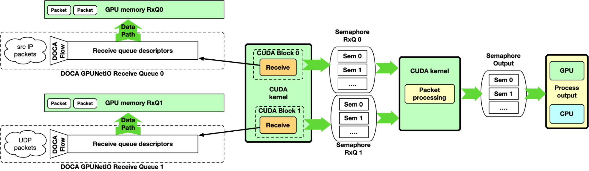
This approach is suitable for high-speed network and latency-sensitive applications because the latency between two receive operations is not delayed by other tasks. It is desirable to associate each CUDA block of the receiver CUDA kernel to a different queue, receiving all packets from all the queues in parallel.
Single-CUDA kernel
Previous implementation may be simplified by having a single CUDA kernel responsible for receiving and processing packets, still dedicating one CUDA block per queue.
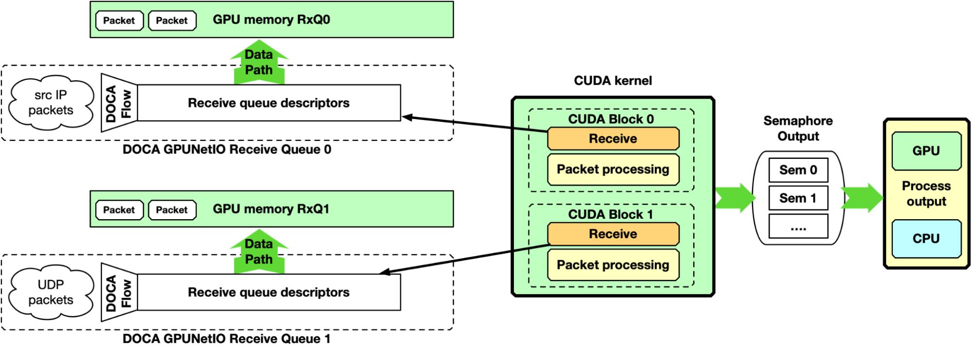
One drawback of this approach is the latency between two receive operations per CUDA block. If packet processing takes a long time, the application may not keep up with receiving new packets in high-speed networks.
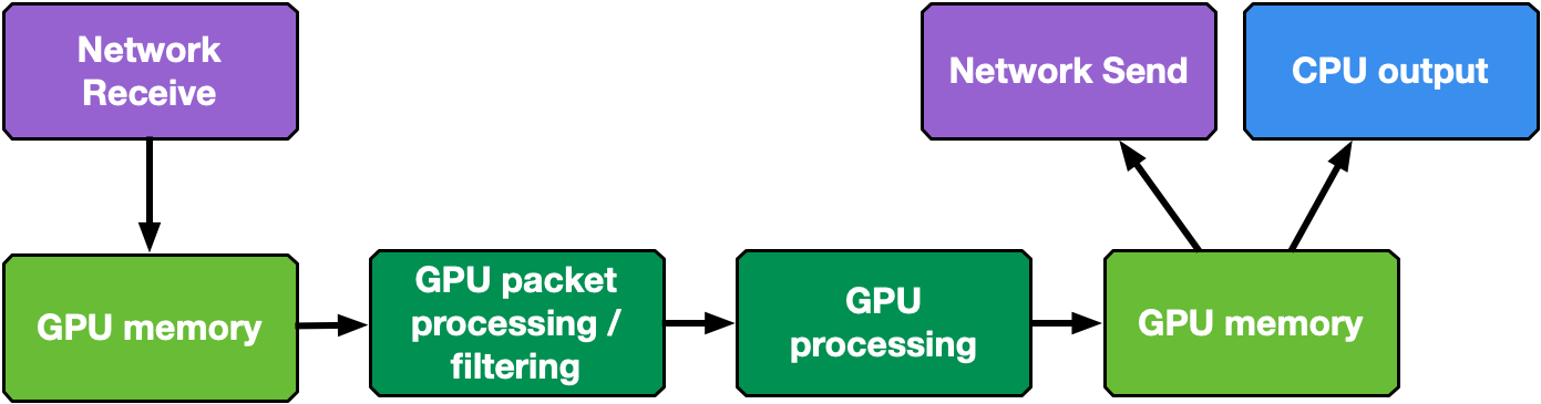
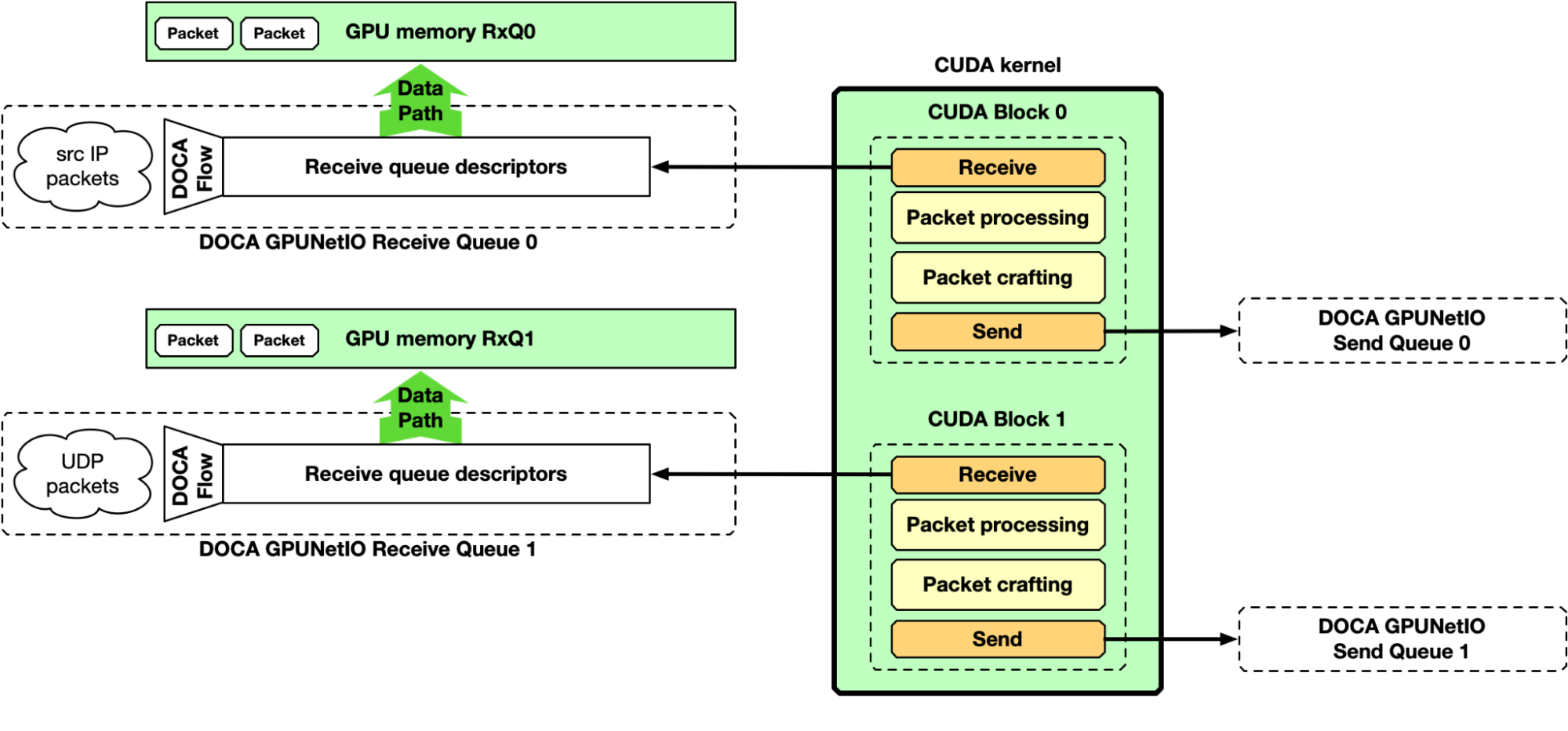
GPU receive, GPU processing, and GPU send
Up to this point, the majority of the focus has been on the “receive and process” part of the pipeline. However, DOCA GPUNetIO also enables the production of some data on the GPU, crafting packets and sending them from a CUDA kernel without CPU intervention. Figure 8 depicts an example of a complete receive, process, and send pipeline.
NVIDIA DOCA GPUNetIO example application
Like any other NVIDIA DOCA library, DOCA GPUNetIO has a dedicated application for API use reference and to test system configuration and performance. The application implements the pipelines described previously, providing different types of packet processing such as IP checksum, HTTP packet filtering, and traffic forward.
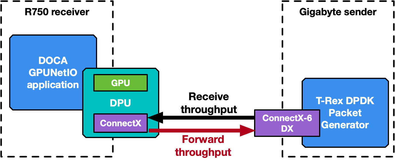
The following section provides an overview of the application’s different modes of operation. Some performance numbers are reported, to be considered as preliminary results that may change and improve in future releases. Two benchmark systems are used, one to receive packets and a second to send packets, connected back-to-back (Figure 9).
The receiver, running the DOCA GPUNetIO application, is a Dell PowerEdge R750 with NVIDIA BlueField-2X DPU converged card. The configuration is embedded CPU mode, so the application runs on the host system CPU using the NIC NVIDIA ConnectX-6 Dx and the GPU A100X from the DPU. Software configuration is Ubuntu 20.04, MOFED 5.8 and CUDA 11.8.
The sender is a Gigabyte Intel Xeon Gold 6240R with a PCIe Gen 3 connection to the NVIDIA ConnectX-6 Dx. This machine does not require any GPU, as it runs the T-Rex DPDK packet generator v2.99. Software configuration is Ubuntu 20.04 with MOFED 5.8.
The application has been executed also on the DPU Arm cores, leading to the same performance result and proving that a GPU-centric solution is platform-independent with respect to the CPU.
Note that the DOCA GPUNetIO minimum requirements are systems with GPU and NIC with a direct PCIe connection. The DPU is not a strict requirement.
IP checksum, GPU receive only
The application creates one or multiple receive queues using GPU-initiated communications to receive packets. Either the single-CUDA kernel or multi-CUDA kernel mode can be used.
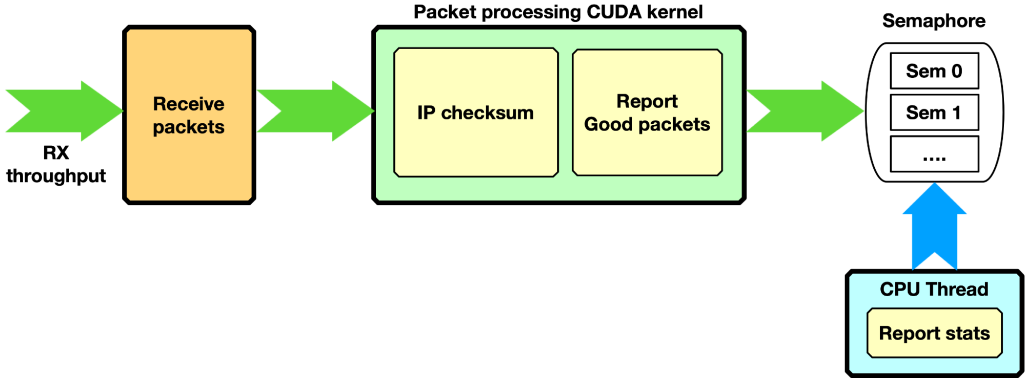
Each packet is processed with a simple IP checksum verification, and only packets passing this test are counted as “good packets.” Through a semaphore, the number of good packets is reported to the CPU, which can print a report on the console.
Zero-packet loss with single queue was achieved by sending with the T-Rex packet generator 3 billion packets of 1 KB size at ~100 Gbps (~11.97 Mpps) and reporting, on the DOCA GPUNetIO application side, the same number of packets with right IP checksum. The same configuration was tested on a BlueField-2 converged card with the same results, proving that GPU-initiated communication is a platform-independent solution.
With a packet size of 512 bytes, T-Rex packet generator was not able to send more than 86 Gbps (~20.9 Mpps). Even with almost twice the number of packets per second, DOCA GPUNetIO did not report any packet drop.
HTTP filtering, GPU receive only
Assuming a more complex scenario, the packet processing CUDA kernel is filtering only HTTP packets with certain characteristics. It copies “good packet” information into a second GPU memory HTTP packets list. As soon as the next item in this HTTP packets list is full of packets, through a dedicated semaphore, the filtering CUDA kernel unblocks a second CUDA kernel to run some inference the HTTP packets accumulated. The semaphore can also be used to report stats to the CPU thread.
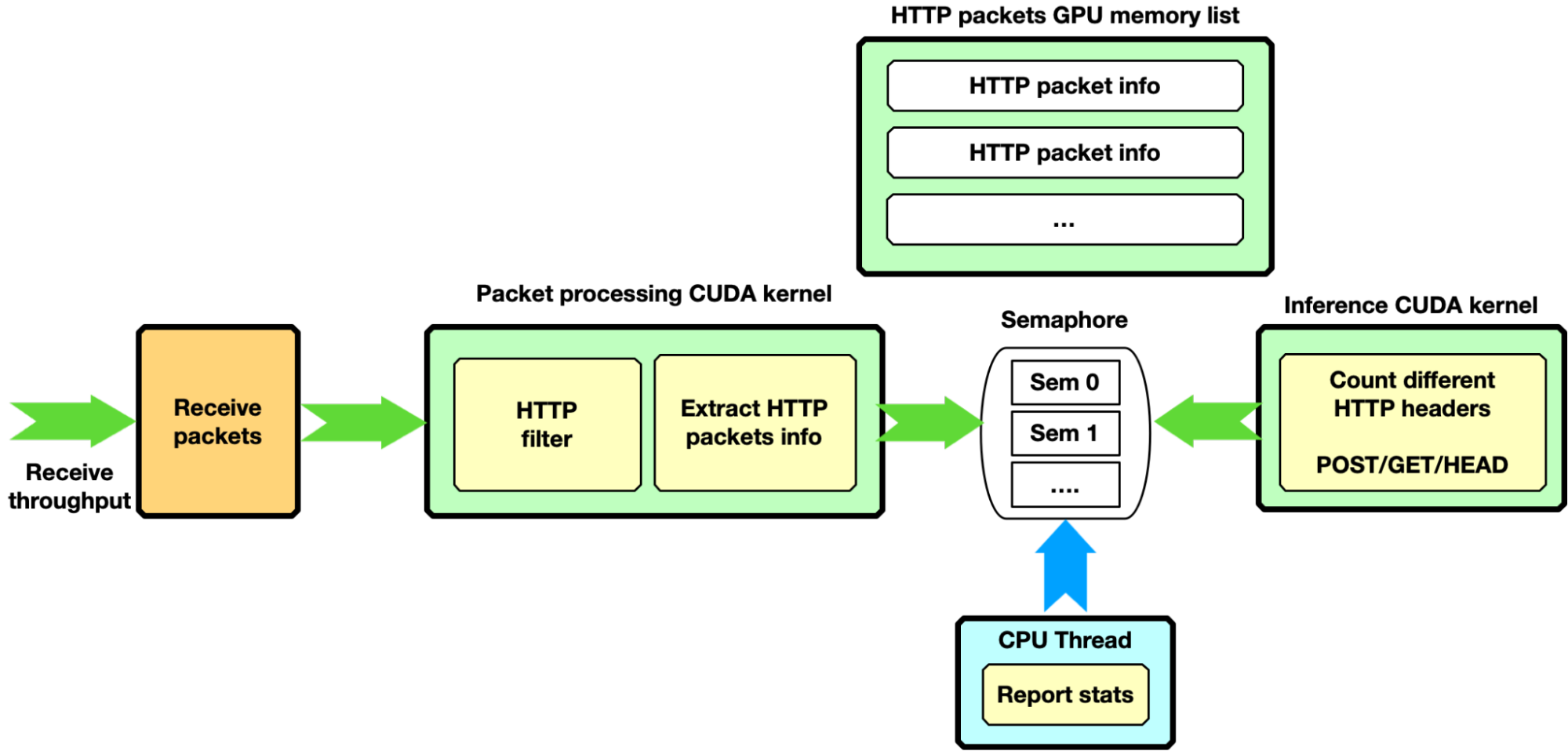
This pipeline configuration provides an example of a complex pipeline comprising multiple stages of data processing and filtering combined with inference functions, such as an AI pipeline.
Traffic forward
This section shows how to enable traffic forwarding with DOCA GPUNetIO with GPU-initiated communications. In each received packet, the MAC and IP source and destination addresses are swapped before sending back packets over the network.
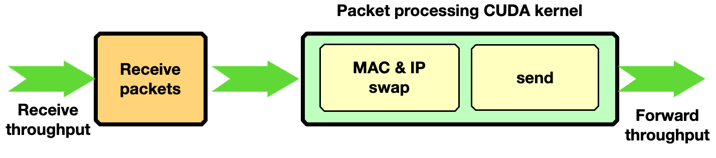
Zero-packet loss with only one receive queue and one send queue was achieved by sending with the T-Rex packet generator 3 billion packets of 1 KB size at ~90 Gbps.
NVIDIA Aerial SDK for 5G
The decision to adopt a GPU-centric solution can be motivated by performance and low-latency requirements, but also to improve system capacity. The CPU may become a bottleneck when dealing with a growing number of peers connecting to the receiver application. The high degree of parallelization offered by the GPU can provide a scalable implementation to handle a great number of peers in parallel without affecting performance.
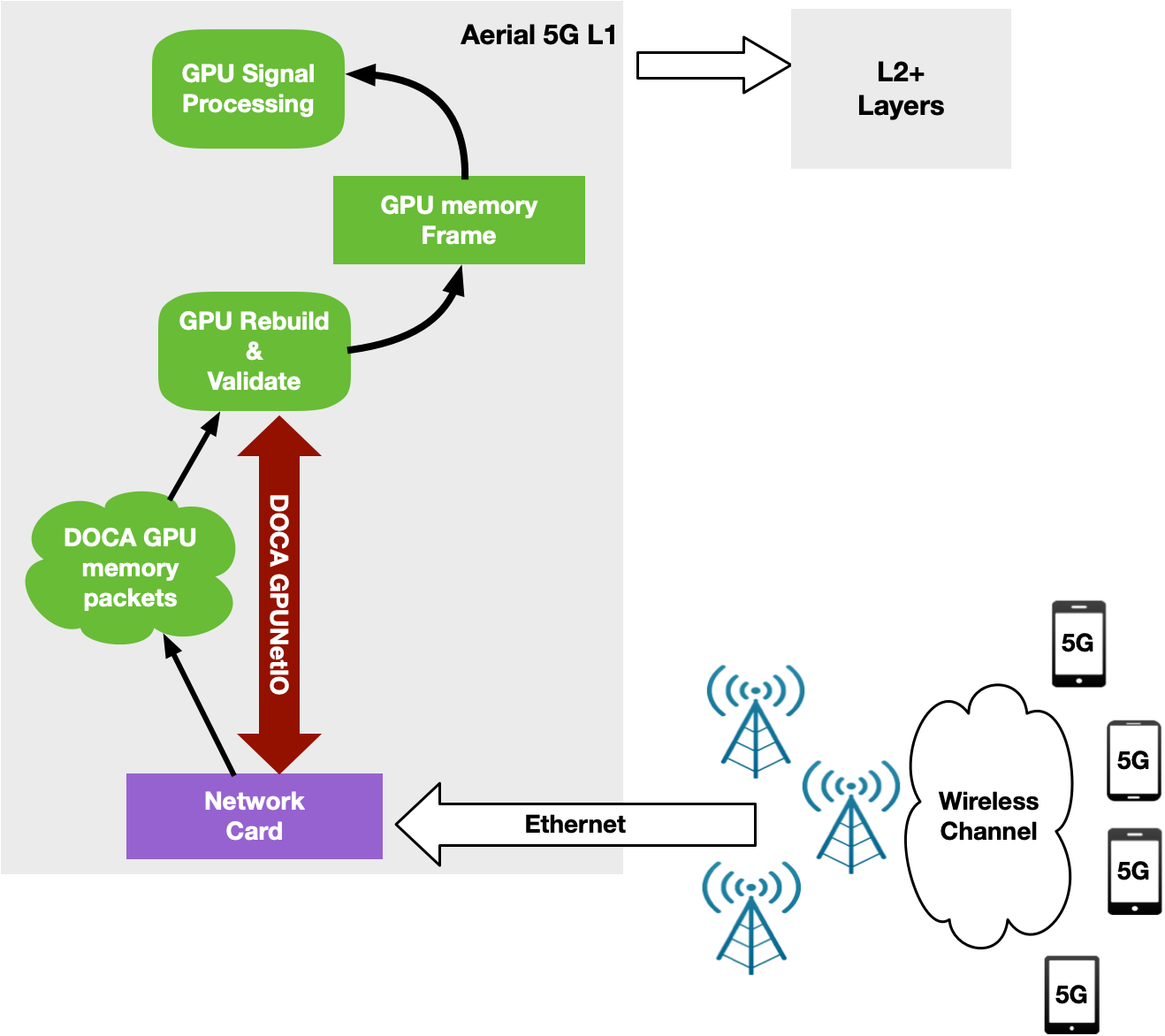
NVIDIA Aerial is an SDK for building a high-performance, software-defined 5G L1 stack optimized with parallel processing on the GPU. Specifically, the NVIDIA Aerial SDK can be used to build the baseband unit (BBU) software responsible to send (Downlink) or receive (Uplink) wireless client data frames split into multiple Ethernet packets through Radio Units (RUs).
In Uplink, BBU receives packets, validates them, and rebuilds the original data frame per RU before triggering the signal processing. With the NVIDIA Aerial SDK, this happens in the GPU: a CUDA kernel is dedicated to each RU per time slot, to rebuild the frame and trigger a sequence of CUDA kernels for GPU signal processing.
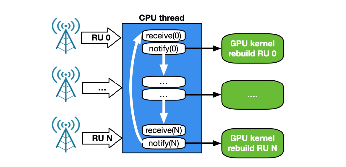
The orchestration of the network card to receive packets and of the GPU to reorder and process packets was implemented through the DPDK gpudev library (Figure 13).

This first implementation was able to keep up with 4 RU working at full 25 Gbps speed using just one CPU core on a modern Intel x86 system. As the number of cells increased, however, the CPU functioning between the network card and the GPU became the bottleneck.
A CPU works in a sequential manner. With a single CPU core to receive and manage traffic for a growing number of RUs, the time between two receives for the same RU depends on the number of RUs. With 2 CPU cores, each working on a subset of RU, the time between two receives for the same RU is halved. However, this approach is not scalable with a growing number of clients. In addition, the magnitude of PCIe transactions increases from NIC to CPU, and then from CPU to GPU (Figure 14).
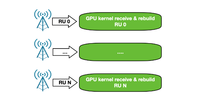
To overcome all of these issues, a new GPU-centric version of the NVIDIA Aerial SDK has been implemented with DOCA GPUNetIO Library. Each CUDA kernel responsible to rebuild, per time slot, the packets coming from a specific RU, has been improved with the receive capability (Figure 15).
At this point, the CPU is not required in the critical path as each CUDA kernel is fully independent, able to process in parallel and in real time a growing number of RUs. This increases system capacity and reduces latency to process packets per slot and number of PCIe transactions. The CPU does not have to communicate with the GPU to provide packet information.
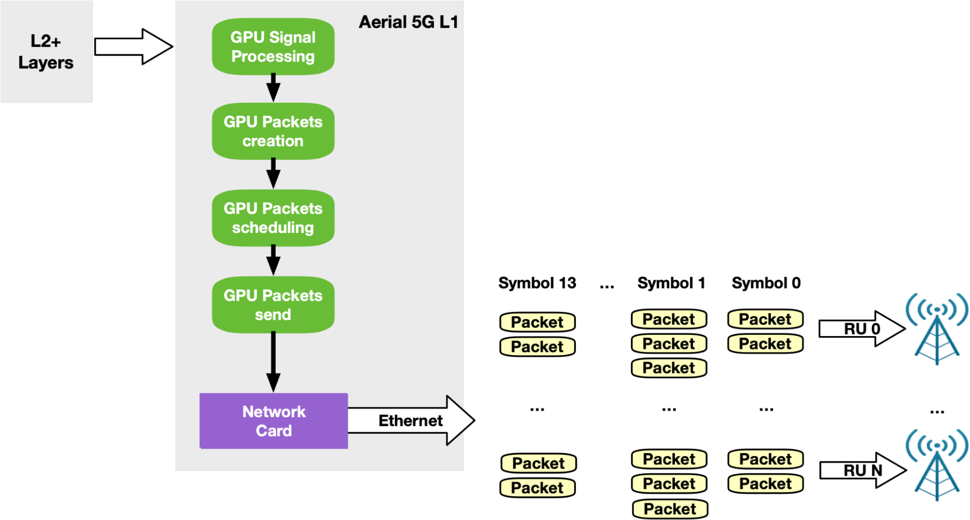
According to the standards, 5G networks must exchange packets according to a specific pattern. Every time slot (500 microseconds, for example), packets should be sent in 14 so-called symbols. Each symbol is composed of a number of packets (depending on the use case) to be sent in a smaller time window (36 microseconds, for example). To support this timed transmission pattern on the Downlink side, the NVIDIA Aerial SDK combines GPU-initiated communications with Accurate Send Scheduling through DOCA GPUNetIO API.
Once GPU signal processing prepares the data to be sent in a future slot, a dedicated CUDA kernel per RU splits this data into Ethernet packets per RU and schedules their future transmission at a specific time in the future. The same CUDA kernel then pushes packets to the NIC that will be responsible for sending each packet at the right time (Figure 17).
Get early access to NVIDIA DOCA GPUNetIO
Created as part of a research project, the DOCA GPUNetIO package is in experimental status. It is available in early access and is an extension of the latest DOCA release. It can be installed on a host system or DPU converged card and includes:
- A set of CPU functions for the initial setup phase of your application that prepare the environment and create the queues and other objects
- A set of GPU-specific functions you can call within your CUDA kernel to send or receive packets and interact with DOCA GPUNetIO semaphores
- An application source code you can build and run to test functionalities and learn about how to use the DOCA GPUNetIO API
Hardware requirements are a ConnectX-6 Dx or newer network card and GPU Volta or newer. It is highly recommended to have a dedicated PCIe bridge between the two. Software requirements are Ubuntu 20.04 or newer, CUDA 11.7 or newer, and MOFED 5.8 or newer.
If you are interested in learning more and gaining hands-on experience with NVIDIA DOCA GPUNetIO to help you develop your next critical application, contact NVIDIA Technical Support for early access. Note that the DOCA GPUNetIO Library is currently only available under NDA with NVIDIA.
 Machine learning operations, MLOps, are best practices for businesses to run AI successfully with help from an expanding smorgasbord of software products and…
 Virtual agents or voice-enabled assistants have been around for quite some time. But in the last decade, their usefulness and popularity have exploded with the…
 According to IDC, the volume of data generated each year is growing exponentially. IDC’s Global DataSphere projects that the world will generate 221 ZB…
 The latest NVIDIA Cybersecurity Hackathon brought together 10 teams to create exciting cybersecurity innovations using the NVIDIA Morpheus cybersecurity AI…


 Learn about the newest CUDA features such as release compatibility, dynamic parallelism, lazy module loading, and support for the new NVIDIA Hopper and NVIDIA…
 The latest version of the NVIDIA TAO Toolkit 4.0 boosts developer productivity with all-new AutoML capability, integration with third-party MLOPs services, and…