
 The Unreal Engine 5.1 release includes cutting-edge advancements that make it easier to incorporate realistic lighting and accelerate graphics workflows. Using…
The Unreal Engine 5.1 release includes cutting-edge advancements that make it easier to incorporate realistic lighting and accelerate graphics workflows. Using the NVIDIA RTX branch of Unreal Engine (NvRTX), you can significantly increase hardware ray-traced and path-traced operations by up to 40%.
Unreal Engine 5.1 features Lumen, a real-time global illumination solution, which enables developers to create more dynamic scenes where indirect lighting changes on the fly. Realistic lighting is an essential component when creating scenes in games, and Lumen can provide high-quality, scalable global illumination and hardware ray-traced reflections.
Nanite, the Unreal Engine (UE) virtualized geometry system, enables film-quality art consisting of billions of polygons to be directly imported into UE, all while maintaining the highest image quality in real time.
In addition to Lumen and Nanite, Unreal Engine 5.1 advances important features that speed up development cycles like Virtual Shadow Maps, Programmable Rasterizer, Virtual Assets, and automated pipeline state object caching for DX12.
NVIDIA is accelerating this new feature set through a combination of NVIDIA RTX 4090, Shader Execution Reordering, and hardware-accelerated ray tracing cores. Thousands of developers have already experienced the benefits of Unreal Engine with NVIDIA technologies. Over the past few years, NVIDIA has delivered GPUs, libraries, and APIs to support the latest features of Unreal Engine.
Next-generation RTX lighting
Achieving the most accurate lighting in computer graphics requires replicating how light physics simulate in the real world. Path-traced lighting has been used in offline rendering in films to achieve physically accurate results. However, that is an expensive and time-consuming process.
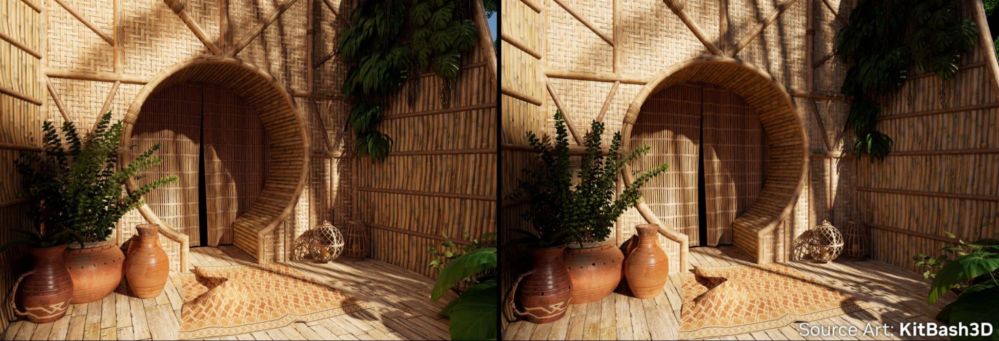
Continued advancements in hardware ray-traced shadows in Unreal Engine 5.1 improve shadow quality using an algorithm that more closely matches offline path tracing. This allows you to create more realistic scenes in real time.
RTX Direct Illumination (RTXDI), available through NvRTX, allows you to take dynamic light counts from single digits into the hundreds. RTXDI uses the same algorithm for direct lighting as the offline path tracer, taking a step closer to unlimited lighting and photorealism.
The next evolution of this technology is in gaming and real-time rendering, which considerably accelerates the time in which frames are processed and rendered.
Shader Execution Reordering
A new technology called Shader Execution Reordering (SER) can help solve the challenge of accurately simulating light. SER provides performance gains in ray tracing operations and optimization for specific use cases. NVIDIA is accelerating real-time ray tracing and offline path tracing by leveraging SER through NvRTX.
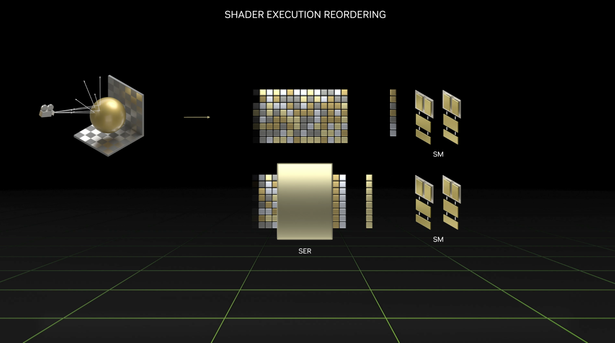
NvRTX features SER integration to support optimization of many of its ray tracing paths. Developers will see additional frame rate optimization on 40 series cards with up to 40% speed increases in ray tracing operations, and zero impact on quality and content authoring. This improves the efficiency of complex ray tracing calculations, and provides greater gains in scenes that take advantage of ray tracing benefits.
Offline path tracing, which is arguably the most complex tracing operation, will see the largest benefit from SER in Unreal Engine 5.1, with speed improvements of 40% or more. Hardware ray-traced reflections and translucency, which have complex interactions with materials and lighting, will also see benefits.
For more information about SER in Unreal Engine 5.1, see the Shader Execution Reordering Whitepaper and Improve Shader Performance and In-Game Frame Rates with Shader Execution Reordering.
Summary
Epic Games and NVIDIA are leading the way into the next generation of rendering, moving the industry toward the future of graphics. With improvement leaps made in each version release of Unreal Engine, developers can expect even more groundbreaking advancements in this space.
Learn more about NVIDIA technologies and Unreal Engine.
 The metaverse is the “next evolution of the internet, the 3D internet,” according to NVIDIA CEO Jensen Huang.