Load times. They are the bane of any developer trying to construct a seamless experience. Trying to hide loading in a game by forcing a player to shimmy…
Load times. They are the bane of any developer trying to construct a seamless experience. Trying to hide loading in a game by forcing a player to shimmy through narrow passages or take extremely slow elevators breaks immersion.
Now, developers have a better solution. NVIDIA collaborated with Microsoft and IHV partners to develop GDeflate for DirectStorage 1.1, an open standard for GPU compression. The current Game Ready Driver (version 526.47) contains NVIDIA RTX IO technology, including optimizations for GDeflate.
GDeflate: An Open GPU Compression Standard
GDeflate is a high-performance, scalable, GPU-optimized data compression scheme that can help applications make use of the sheer amount of data throughput available on modern NVMe devices. It makes streaming decompression from such devices practical by eliminating CPU bottlenecks from the overall I/O pipeline. GDeflate also provides bandwidth amplification effects, further improving the effective throughput of the I/O subsystem.
GDeflate Open Source will be released on GitHub with a permissive license for IHVs and ISVs. We want to encourage the quick embrace of GDeflate as a data-parallel compression standard, facilitating its adoption across the PC ecosystem and on other platforms.
To show the benefits of GDeflate, we measured system performance without compression, with standard CPU-side decompression, and with GPU-accelerated GDeflate decompression on a representative game-focused dataset, containing texture and geometry data.
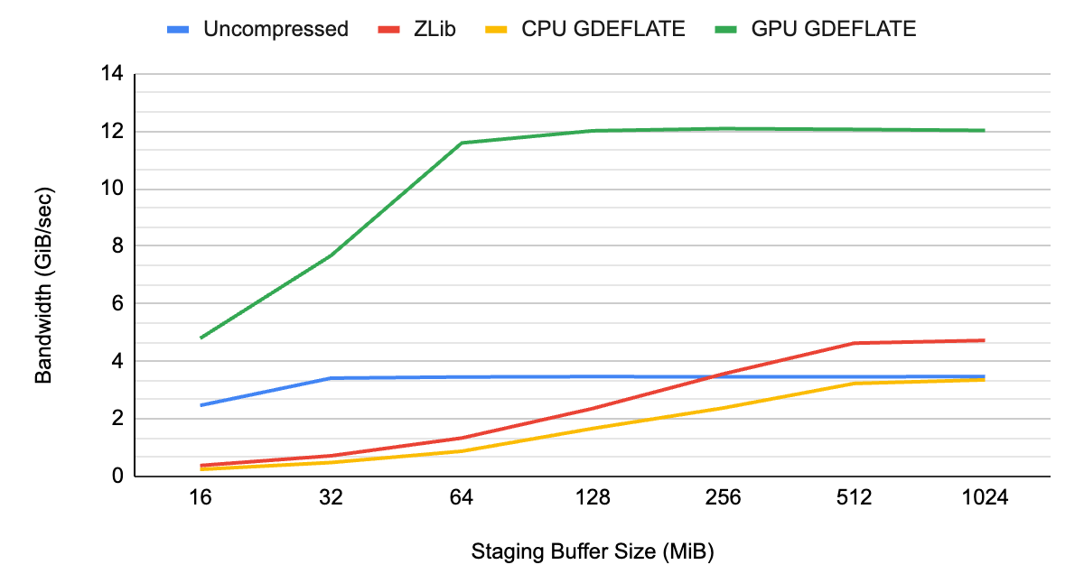
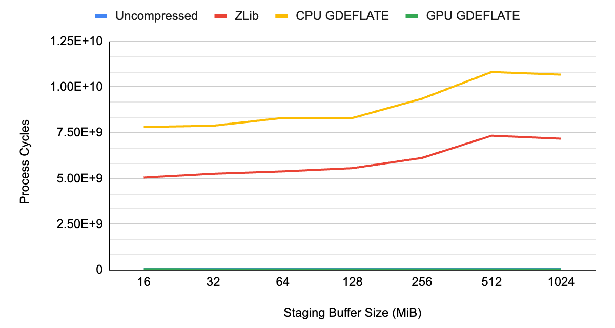
As you can see from Figures 1 and 2, the data throughput of uncompressed streaming is limited by the system bus bandwidth at about ~3 GB/s, which happens to be the limit of a Gen3 PCIe interconnect.
When applying traditional compression with decompression happening on the CPU, it’s the CPU that becomes the overall bottleneck, resulting in lower throughput than would otherwise be possible with uncompressed streaming. Not only does it underutilize available I/O resources of the system, but it also takes away CPU cycles from other tasks needing CPU resources.
With GPU-accelerated GDeflate decompression, the system can deliver effective bandwidth well in excess of what’s possible without applying compression. It is effectively multiplying data throughput by its compression ratio. The CPU remains fully available for performing other important tasks, maximizing system-level performance.
GDeflate is available as a standard GPU decompression option in DirectStorage 1.1—a modern I/O streaming API from Microsoft. We’re looking forward to next-generation game engines benefiting from GDeflate by dramatically reducing loading times.
Resource streaming and data compression
Today’s video games feature extremely detailed interactive environments, requiring the management of enormous assets. This data must be delivered first to the end user’s system, and then, at runtime, actively streamed to the GPU for processing. The bulk of a game’s content package is made up of resources that naturally target the GPU: textures, materials, and geometry data.
Traditional data compression techniques are applicable to game content that rarely changes. For example, a texture that is authored only one time may have to be loaded multiple times as the player advances through a game level. Such assets are usually compressed when they are packaged for distribution and decompressed on demand when the game is played. It has become standard practice to apply compression to game assets to reduce the size of the downloadable (and its installation footprint).
However, most data compression schemes are designed for CPUs and assume serial execution semantics. In fact, the process of data compression is usually described in fundamentally serial terms: a stream of data is scanned serially while looking for redundancies or repeated patterns. It replaces multiple occurrences of such patterns with a reference to their previous occurrence. As a result, such algorithms can’t easily scale to data-parallel architectures or accommodate the need for faster decompression rates demanded by modern game content.
At the same time, recent advances in I/O technology have dramatically improved available I/O bandwidth on the end user system. It’s typical to see a consumer system equipped with a PCIe Gen3 or Gen4 NVMe device, capable of delivering up to 7 GB/s of data bandwidth.
To put this in perspective, at this rate, it is possible to fill the entire 24 GBs of frame buffer memory on the high-end NVIDIA GeForce RTX 4090 GPU in a little over 3 seconds!
To keep up with these system-level I/O speed improvements, we need dramatic advances in data compression technology. At these rates, it is no longer practical to use the CPU for data decompression on the end user’s system. That requires an unacceptably large fraction of precious CPU cycles to be spent on this auxiliary task. It may also slow down the entire system.
The CPU shouldn’t become the bottleneck that holds back the I/O subsystem.
Data-parallel decompression and GDeflate architecture
With Moore’s law ending, we can no longer expect to get “free” performance improvements from serial processors.
High-performance systems have long embraced large-scale data parallelism to continue scaling performance for many applications. On the other hand, parallelizing the traditional data compression algorithms has been challenging, due to fundamental serial assumptions “baked” into their design.
What we need is a GPU-friendly data compression approach that can scale performance as GPUs become wider and more parallel.
This is the problem that we set out to address with GDeflate, a novel data-parallel compression scheme optimized for high-throughput GPU decompression. We designed GDeflate with the following goals:
- High-performance GPU-optimized decompression to support the fastest NVMe devices
- Offload the CPU to avoid making it the bottleneck during I/O operations
- Portable to a variety of data-parallel architectures, including CPUs and GPUs
- Can be implemented cheaply in fixed-function hardware, using existing IP
- Establish as a data-parallel data compression standard
As you could guess from its name, GDeflate builds upon the well-established RFC 1951 DEFLATE algorithm, expanding and adapting it for data-parallel processing. While more sophisticated compression schemes exist, the simplicity and robustness of the original DEFLATE data coding make it an appealing choice for highly tuned GPU-based implementations.
Existing fixed-function implementations of DEFLATE can also be easily adapted to support GDeflate for improved compatibility and performance.
Two-level parallelism
A many-core SIMD machine consumes the GDeflate bitstream by design, explicitly exposing parallelism at two levels.
First, the original data stream is segmented into 64 KB tiles, which are processed independently. This coarse-grained decomposition provides thread-level parallelism, enabling multiple tiles to be processed concurrently on multiple cores of the target processor. This also enables random access to the compressed data at tile granularity. For example, a streaming engine may request a sparse set of tiles to be decompressed in accordance with the required working set for a given frame.
Also, 64 KB happens to be the standard tile size for tiled or sparse resources in graphics APIs (DirectX and Vulkan), which makes GDeflate compatible with future on-demand streaming architectures leveraging these API features.
Second, the bitstream within tiles is specifically formatted to expose finer-grained, SIMD-level parallelism. We expect that a cooperative group of threads will process individual tiles, as the group can directly parse the GDeflate bitstream using hardware-accelerated data-parallel operations, commonly available on most SIMD architectures.
All threads in the SIMD group share the decompression state. The formatting of the bitstream is carefully constructed to enable highly optimized cooperative processing of compressed data.
This two-level parallelization strategy enables GDeflate implementations to scale easily across a wide range of data-parallel architectures, also providing necessary headroom for supporting future, even wider data-parallel machines without compromising decompression performance.
NVIDIA RTX IO supports DirectStorage 1.1
NVIDIA RTX IO is now included in the current Game Ready Driver (version 526.47), which offers accelerated decompression throughput.
Both DirectStorage and RTX IO leverage the GDeflate compression standard.
“Microsoft is delighted to partner with NVIDIA to bring the benefits of next-generation I/O to Windows gamers. DirectStorage for Windows will enable games to leverage NVIDIA’s cutting-edge RTX IO and provide game developers with a highly efficient and standard way to get the best possible performance from the GPU and I/O system. With DirectStorage, game sizes are minimized, load times reduced, and virtual worlds are free to become more expansive and detailed, with smooth and seamless streaming.”
Bryan Langley, Group Program Manager for Windows Graphics and Gaming
Getting started with DirectStorage in RTX IO drivers
We have a few more recommendations to help ensure the best possible experience using DirectStorage with GPU decompression on NVIDIA GPUs.
Preparing your application for DirectStorage
Achieving maximum end-to-end throughput with DirectStorage with GPU decompression requires enqueuing a sufficient number of read requests, to keep the pipeline fully saturated.
In preparation for DirectStorage integration, applications should group resource I/O and creation requests close together in time. Ideally, resource I/O and creation operations occur in their own CPU thread, separate from threads doing other loading screen activities like shader creation.
Assets on disk should be also packaged together in large enough chunks so that DirectStorage API call frequency is kept to a minimum and CPU costs are minimized. This ensures that enough work can be submitted to DirectStorage to keep the pipeline fully saturated.
For more information about general best practices, see Using DirectStorage and the DirectStorage 1.1 Now Available Microsoft post.
Deciding the staging buffer size
- Make sure to change the default staging buffer size whenever GPU decompression is used. The current 32 MB default isn’t sufficient to saturate modern GPU capabilities.
- Make sure to benchmark different platforms with varying NVMe, PCIe, and GPU capabilities when deciding on the staging buffer size. We found that a 128-MB staging buffer size is a reasonable default. Smaller GPUs may require less and larger GPUs may require more.
Compression ratio considerations
- Make sure to measure the impact that different resource types have on compression savings and GPU decompression performance.
- In general, various data types, such as texture and geometry, compress at different ratios. This can cause some variation in GPU decompression execution performance.
- This won’t have a significant effect on end-to-end throughput. However, it may result in variation in latency when delivering the resource contents to their final locations.
Windows File System
- Try to keep disk files accessed by DirectStorage separate from files accessed by other I/O APIs. Shared file use across different I/O APIs may result in the loss of bypass I/O improvements.
Command queue scheduling when background streaming
- In Windows 10, command queue scheduling contention can occur between DirectStorage copy and compute command queues, and application-managed copy and compute command queues.
- The NVIDIA Nsight Systems, PIX, and GPUView tools can assist in determining whether background streaming with DirectStorage is in contention with important application-managed command queues.
- In Windows 11, overlapped execution between DirectStorage and application command queues is fully expected.
- If overlapped execution results in suboptimal performance of application workloads, we recommend throttling back DirectStorage reads. This helps maintain critical application performance while background streaming is occurring.
Summary
Next-generation game engines require streaming huge amounts of data, aiming to create increasingly realistic, detailed game worlds. Given that, it’s necessary to rethink game engines’ resource streaming architecture, and fully leverage improvements in I/O technology.
Using the GPU as an accelerator for compute-intensive, data decompression becomes critical for maximizing system performance and reducing load times.
The NVIDIA RTX IO implementation of GDeflate is a scalable GPU-optimized compression technology that enables applications to benefit from the computational power of the GPU for I/O acceleration. It acts as a bandwidth amplifier for high-performance I/O capabilities of today and future systems.
 Storytelling with data is a crucial soft skill for AI and data professionals. To ensure that stakeholders understand the technical requirements, value, and…

 Large language models (LLMs) are some of the most advanced deep learning algorithms that are capable of understanding written language. Many modern LLMs are…
 GNNs apply the predictive power of deep learning to rich data structures that depict objects and their relationships as points connected by lines in a graph.
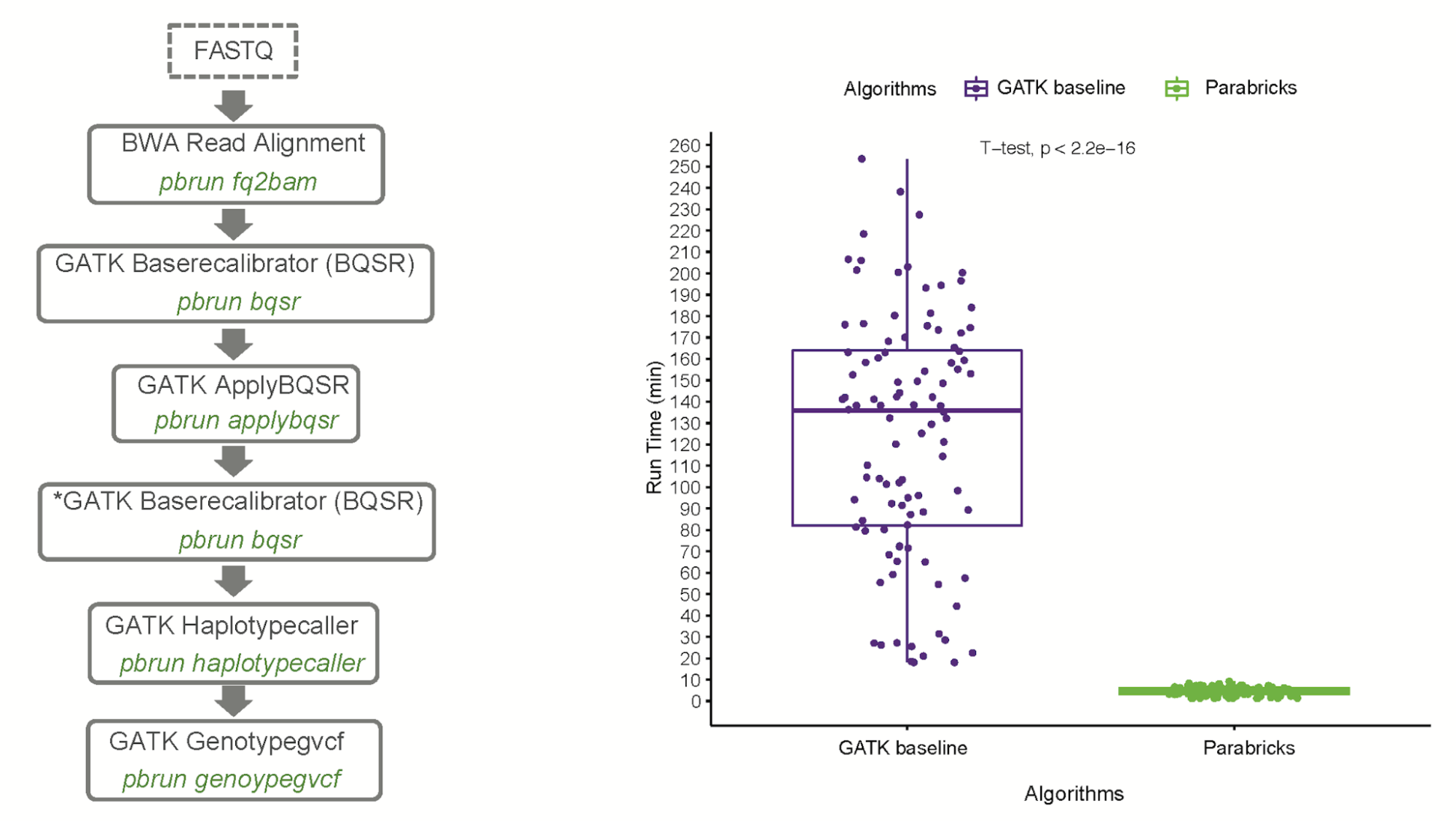
 Many organizations are using Clara Parabricks for fast human genome and exome analysis for large population projects, critically-ill patients, clinical…