The latest NVIDIA HPC SDK update expands portability and now supports the Arm-based AWS Graviton3 processor. In this post, you learn how to enable Scalable…
The latest NVIDIA HPC SDK update expands portability and now supports the Arm-based AWS Graviton3 processor. In this post, you learn how to enable Scalable Vector Extension (SVE) auto-vectorization with the NVIDIA compilers to maximize the performance of HPC applications running on the AWS Graviton3 CPU.
NVIDIA HPC SDK
The NVIDIA HPC SDK includes the proven compilers, libraries, and software tools essential to maximizing developer productivity and building HPC applications for GPUs, CPUs, or the cloud.
NVIDIA HPC compilers enable cross-platform C, C++, and Fortran programming for NVIDIA GPUs and multicore Arm, OpenPOWER, or x86-64 CPUs. These are ideal for HPC modeling and simulation applications written in C, C++, or Fortran with OpenMP, OpenACC, and CUDA.
For example, SPEC CPU® 2017 benchmark scores are estimated to increase by 17% on the AWS Graviton 3 when compiled with the NVIDIA HPC compilers vs. GCC 12.1.
| Speedup (est.) | Ratio (est.) | Seconds (est.) |
|||
| NVHPC | GC1 12.1 | NVHPC | GCC 12.1 | ||
| 64 Copy FPRate | 1.04 | 263 | 254 | 501 | 519 |
| 64 Thread FPSpeed | 1.17 | 188 | 161 | 73.6 | 85.9 |
The compilers are also fully interoperable with the optimized NVIDIA math libraries, communication libraries, and performance tuning and debugging tools. These accelerated math libraries maximize performance on common HPC algorithms, and the optimized communications libraries enable standards-based scalable systems programming.
The integrated performance profiling and debugging tools simplify porting and optimization of HPC applications, and the containerization tools enable easy deployment on-premises or in the cloud.
Arm and AWS Graviton3
AWS Graviton3 launched in May 2022 as the Arm-based CPU from AWS. The Arm architecture has a legacy of power efficiency and support for high memory bandwidth that makes it ideal for cloud and data center computing. Amazon reports:
The Amazon EC2 C7g instances, powered by the latest generation AWS Graviton3 processors, provide the best price performance in Amazon EC2 for compute-intensive workloads. C7g instances are ideal for HPC, batch processing, electronic design automation (EDA), gaming, video encoding, scientific modeling, distributed analytics, CPU-based machine learning (ML) inference, and ad-serving. They offer up to 25% better performance over the sixth generation AWS Graviton2-based C6g instances.
Compared to AWS Graviton2, ANSYS benchmarked 35% better performance on AWS Graviton3. Formula 1 simulations are also 40% faster. Arm-based CPUs have been delivering significant innovations and performance enhancements since the launch of the Arm Neoverse product line, when the Neoverse N1 core exceeded performance expectations by 30%.
In keeping with the history of Arm enabling support for new computing technologies well ahead of the competition, AWS Graviton3 features DDR5 memory and the SVE to the Arm architecture.
Amazon EC2 C7g instances are the first in the cloud to feature DDR5 memory, which provides 50% higher memory bandwidth compared to DDR4 memory to enable high-speed access to data in memory. The best way to take full advantage of all that memory bandwidth is to use the latest in vectorization technologies: Arm SVE.
SVE architecture
In addition to being the first cloud-hosted CPU to offer DDR5, AWS Graviton3 is also the first in the cloud to feature SVE.
SVE was first introduced in the Fujitsu A64FX CPU, which powers the RIKEN Fugaku supercomputer. When Fugaku launched, it shattered all contemporary HPC CPU benchmarks and placed confidently at the top of the TOP500 supercomputers list for two years.
SVE and high-bandwidth memory are the key design features of the A64FX that make it ideal for HPC, and both these features are present in the AWS Graviton3 processor.
SVE is a next-generation SIMD extension to the Arm architecture. It enables flexible vector length implementations with a range of possible values in CPU implementations. The vector length can vary from a minimum of 128 bits to a maximum of 2,048 bits, at 128-bit increments.
For example, the Fujitsu A64FX implements SVE at 512-bits, while AWS Graviton3 implements it at 256-bits. Unlike other SIMD architectures, the same assembly code runs on both CPUs, even though the hardware vector bit-width is different. This is called vector-length agnostic (VLA) programming.
VLA code is highly portable and can enable compilers to generate better assembly code. But, if a compiler knows the target CPU’s hardware vector bit-width, it can enable further optimizations for that specific architecture. This is vector length–specific (VLS) programming.
SVE uses the same assembly language for both VLA and VLS. The only difference is that the compiler is free to make additional assertions about data layout, loop trip counts, and other relevant features while generating the code. This results in highly optimized, target-specific code that takes full advantage of the CPU.
SVE also introduces a powerful range of advanced features ideal for HPC and ML applications:
- Gather-load and scatter-store instructions allow operations on arrays-of-structures and other noncontiguous data to vectorize.
- Speculative vectorization enables the SIMD acceleration of string manipulation functions and loops that contain control flow.
- Horizontal and serialized vector operations facilitate data reductions and help optimize loops processing large datasets.
SVE is not an extension or the replacement of the NEON instruction set, which is also available in AWS Gravition3. SVE is redesigned for better data parallelism for HPC and ML.
Maximizing Graviton3 performance with NVIDIA HPC compilers
Compiler auto-vectorization is one of the easiest ways to take advantage of SVE, and the NVIDIA HPC compilers add support for SVE auto-vectorization in the 22.7 release.
To maximize performance, the compiler performs analysis to determine which SIMD instructions to generate. SVE auto-vectorization uses target-specific information to generate highly optimized vector length–specific (VLS) code based on the vector bit-width of the CPU core.
To enable SVE auto-vectorization, specify the appropriate -tp architecture flag for the target CPU: -tp=neoverse-v1. Not specifying a -tp option assumes that the application will be executed on the same system on which it was compiled.
Applications compiled with the NVIDIA HPC compilers on Graviton3 automatically take full advantage of the CPU’s 256-bit SVE SIMD units. Graviton3 is also backward compatible with the -tp=neoverse-n1 option but only runs vector code on its 128-bit NEON SIMD units.
Getting started with the NVIDIA HPC SDK
The NVIDIA HPC SDK provides a comprehensive and proven software stack. It enables HPC developers to create and optimize application performance on high-performance systems such as the NVIDIA platform and AWS Graviton3.
By providing a wide range of programming models, libraries, and development tools, applications can be efficiently developed for the specialized hardware that enables state-of-the-art performance in systems such as NVIDIA GPUs and SVE-enabled processors like AWS Graviton3.
For more information, see the following resources:
- Learn more about the compiler support and other posts at HPC SDK.
- Download the HPC SDK software for free.
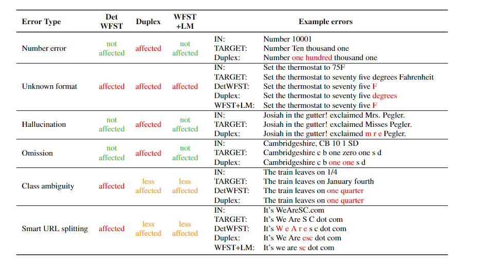
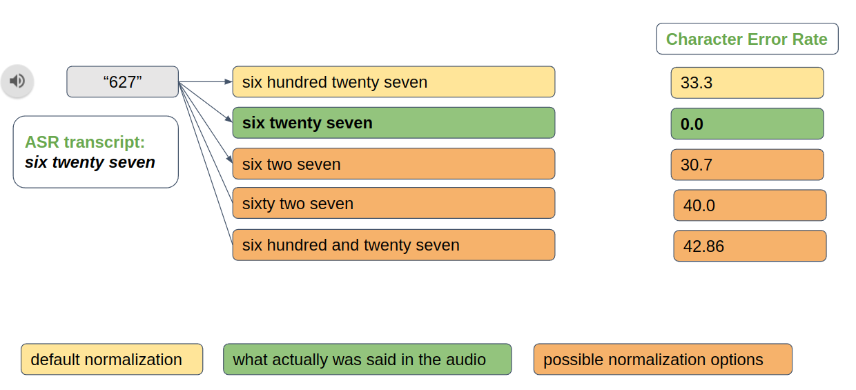
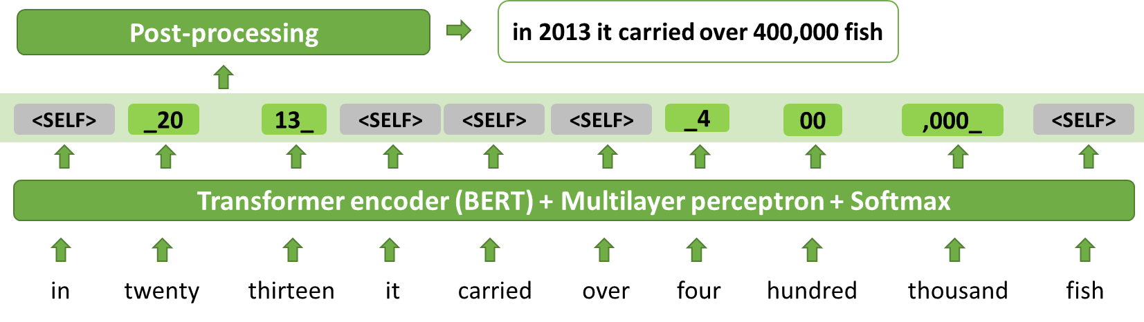
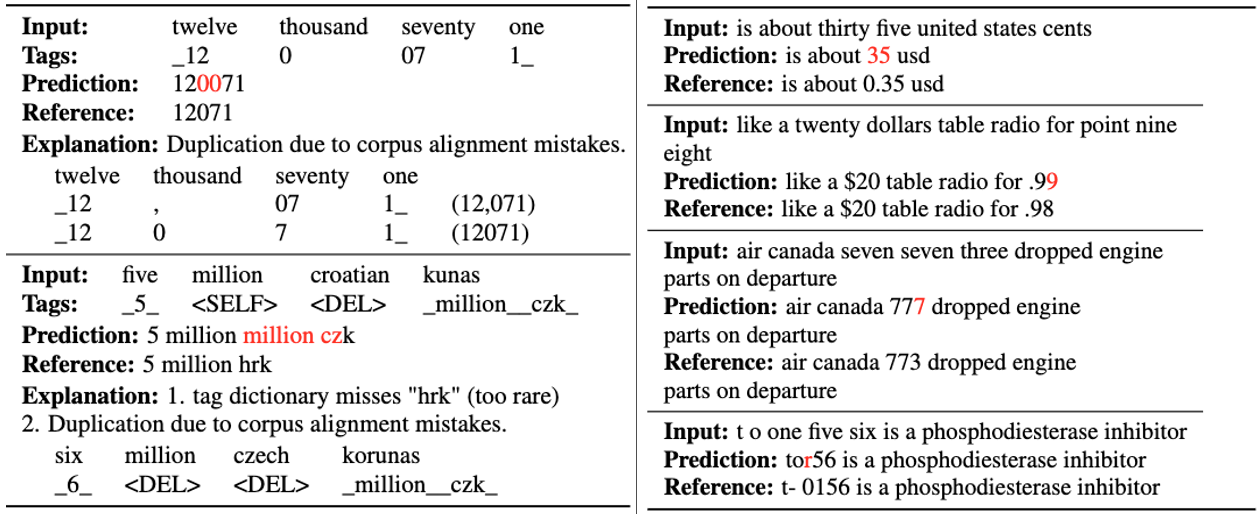
 Text normalization (TN) converts text from written form into its verbalized form, and it is an essential preprocessing step before text-to-speech (TTS). TN…
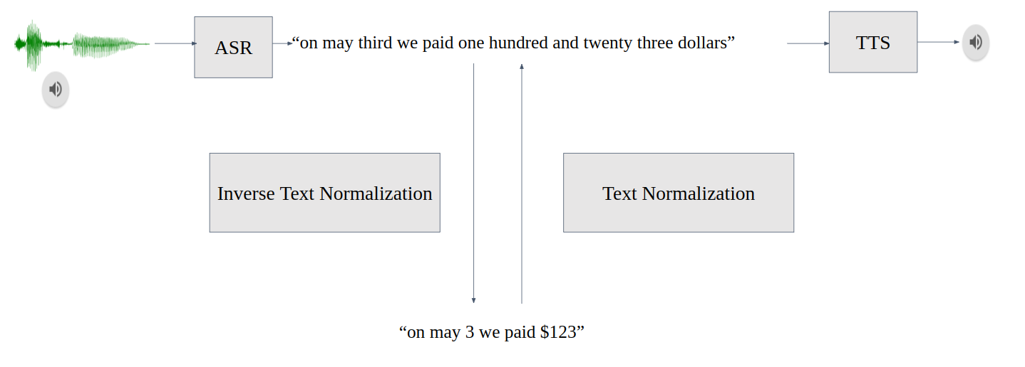

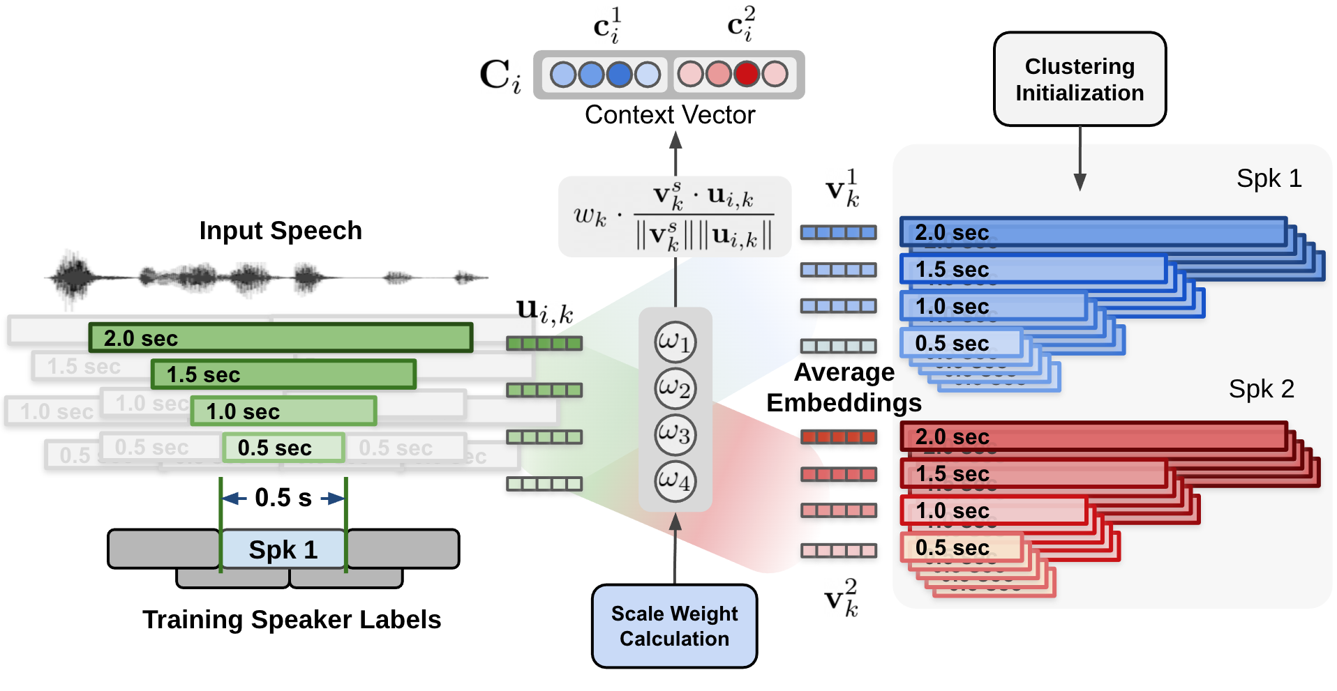
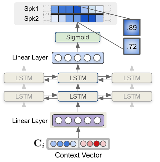
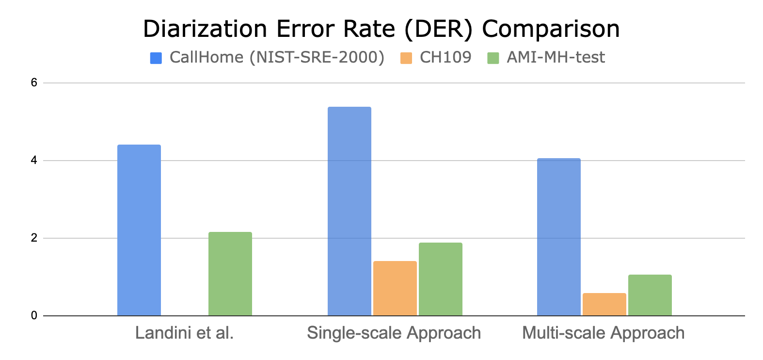
 Speaker diarization is the process of segmenting audio recordings by speaker labels and aims to answer the question “Who spoke when?”. It makes a clear…
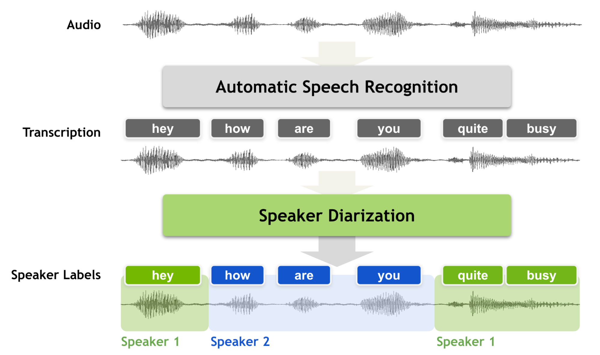


 Learn about new CUDA features, digital twins for weather and climate, quantum circuit simulations, and much more with these GTC 2022 sessions.
  There is an abundance of market-approved medical AI software that can be used to improve patient care and hospital operations, but we have not yet seen these…
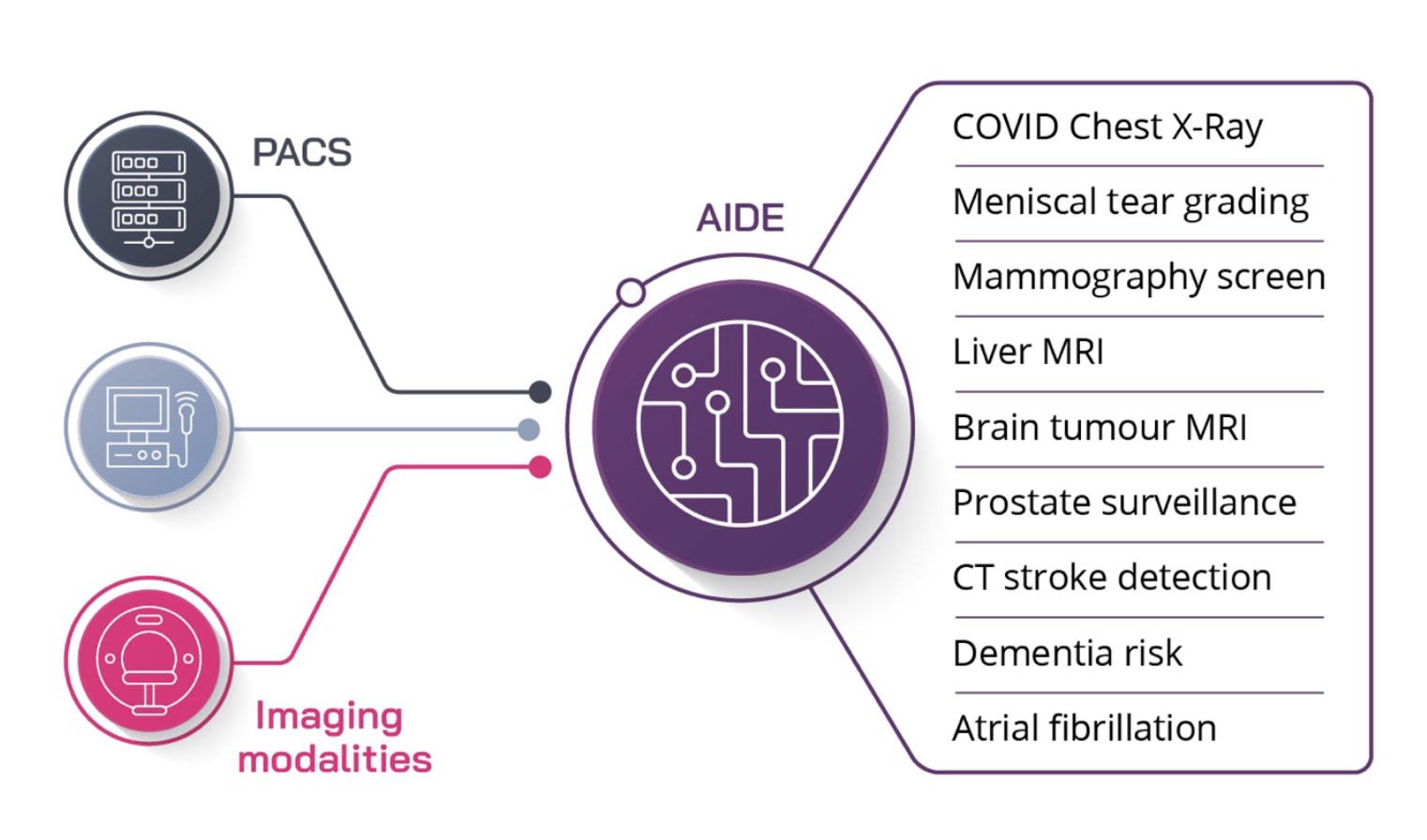