 The latest version of CUTLASS offers users BLAS3 operators accelerated by tensor cores, Python integrations, GEMM compatibility extensions, and more.
Categories
 DataBloom
The latest version of CUTLASS offers users BLAS3 operators accelerated by tensor cores, Python integrations, GEMM compatibility extensions, and more.
Thanks to the GeForce cloud, even Mac users can be PC gamers. This GFN Thursday, fire up your Macbook and get your game on. This week brings eight more games to the GeForce NOW library. Plus, members can play Genshin Impact and claim a reward to start them out on their journeys streaming on GeForce Read article >
The post Making an Impact: GFN Thursday Transforms Macs Into GeForce Gaming PCs appeared first on NVIDIA Blog.
A camera begins in the sky, flies through some trees and smoothly exits the forest, all while precisely tracking a car driving down a dirt path. This would be all but impossible in the real world, according to film and photography director Brett Danton.
The post Meet the Omnivore: Director of Photography Revs Up NVIDIA Omniverse to Create Sleek Car Demo appeared first on NVIDIA Blog.
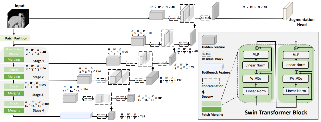
 The NVIDIA Swin UNETR model is the first attempt for large-scale transformer-based self-supervised learning in 3D medical imaging.
At the Computer Vision and Pattern Recognition Conference (CVPR), NVIDIA researchers are presenting over 35 papers. This includes work on Shifted WINdows UNEt TRansformers (Swin UNETR)—the first transformer-based pretraining framework tailored for self-supervised tasks in 3D medical image analysis. The research is the first step in creating pretrained, large-scale, and self-supervised 3D models for data annotation.
As a transformer-based approach for computer vision, Swin UNETR employs MONAI, an open-source PyTorch framework for deep learning in healthcare imaging, including radiology and pathology. Using this pretraining scheme, Swin UNETR has set new state-of-the-art benchmarks for various medical image segmentation tasks and consistently demonstrates its effectiveness even with a small amount of labeled data.
The Swin UNETR model was trained on an NVIDIA DGX-1 cluster using eight GPUs and the AdamW optimization algorithm. It was pretrained on 5,050 publicly available CT images from various body regions of healthy and unhealthy subjects selected to maintain a balanced dataset.
For self-supervised pretraining of the 3D Swin Transformer encoder, the researchers used a variety of pretext tasks. Randomly cropped tokens were augmented with different transforms such as rotation and cutout. These tokens were used for masked volume inpainting, rotation, and contrastive learning, for the encoder to learn a contextual representation of training data, without increasing the burden of data annotation.
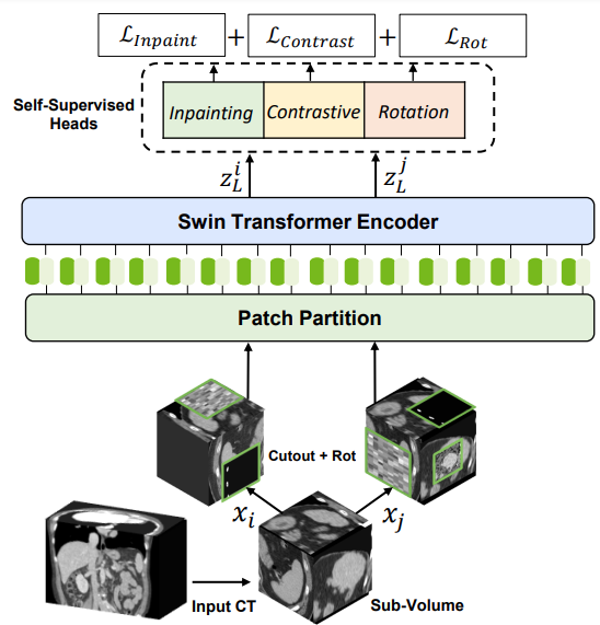
Swin Transformers adopts a hierarchical Vision Transformer (ViT) for local computing of self-attention with nonoverlapping windows. This unlocks the opportunity to create a medical-specific ImageNet for large companies and removes the bottleneck of needing a large quantity of high-quality annotated datasets for creating medical AI models.
Compared to CNN architectures, the ViT demonstrates exceptional capability in self-supervised learning of global and local representations from unlabeled data (the larger the dataset, the stronger the pretrained backbone). The user can fine-tune the pretrained model in downstream tasks (for example, segmentation, classification, and detection) with a very small amount of labeled data.
This architecture computes self attention in local windows and has shown better performance in comparison to ViT. In addition, the hierarchical nature of Swin Transformers makes them well suited for tasks requiring multiscale modeling.
Following the success of the pioneering UNETR model with a ViT-based encoder that directly uses 3D patch embeddings, Swin UNETR uses a 3D Swin Transformer encoder with a pyramid-like architecture.
In the encoder of the Swin UNETR, self-attention is computed in local windows since computing naive global self-attention is not feasible for high-resolution feature maps. In order to increase the receptive field beyond the local windows, window-shifting is used to compute the region interaction for different windows.
The encoder of the Swin UNETR is connected to a residual UNet-like decoder at five different resolutions by skip connections. It can capture multiscale feature representations for dense prediction tasks, such as medical image segmentation.
After fine-tuning with the Beyond the Cranial Vault (BTCV) Segmentation Challenge on 13 abdominal organs in CT and the segmentation tasks from the Medical Segmentation Decathlon (MSD) dataset, the model achieved state-of-the-art accuracy on the public leaderboards.
In the BTCV, Swin UNETR obtained an average Dice of 0.918, outperforming other top-ranked models.
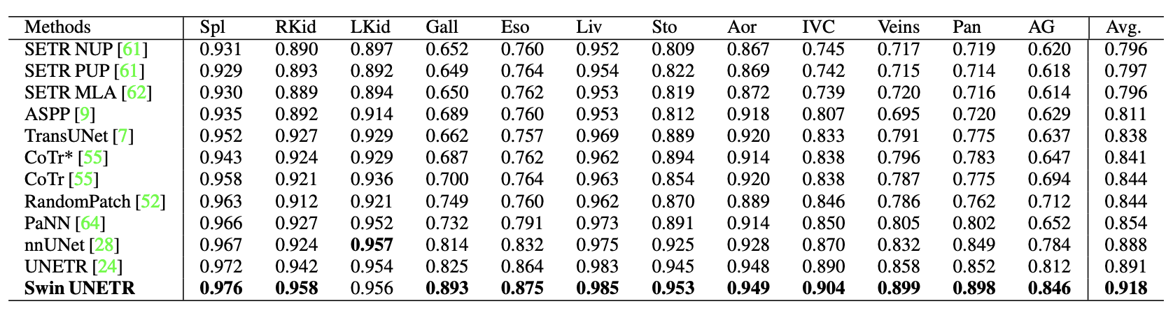
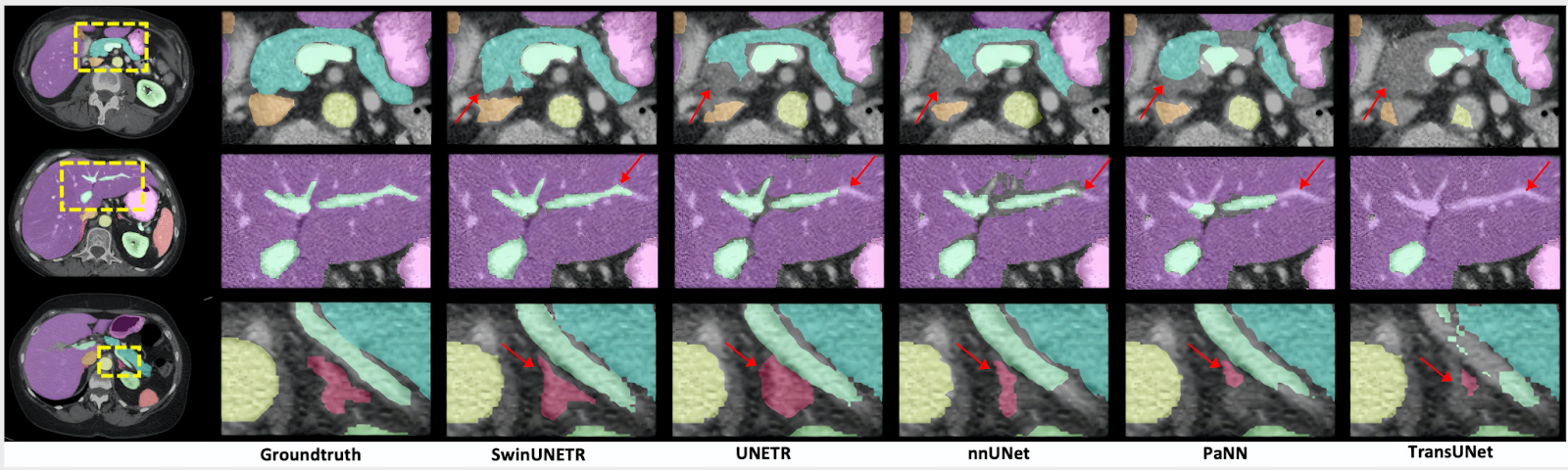
There are improvements compared to prior state-of-the-art methods for smaller organs, such as the splenic and portal veins (3.6%), pancreas (1.6%), and adrenal glands (3.8%.) Small organ data label segmentation is an excruciatingly difficult task for a radiologist. The improvement can be seen in the figure below.
In the MSD, Swin UNETR achieved state-of-the-art performance in brain tumor, lung, pancreas, and colon. The results are comparable for the heart, liver, hippocampus, prostate, hepatic vessel, and spleen. Overall, Swin UNETR presented the best average Dice of 78.68% across all 10 tasks and achieved the top ranking on the MSD leaderboard.
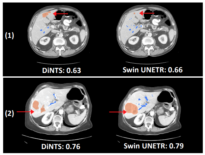
Swin UNETR has shown better segmentation performance using significantly fewer training GPU hours compared to DiNTS—a powerful AutoML methodology for medical image segmentation. For instance, qualitative segmentation outputs for the task of hepatic vessel segmentation demonstrate the capability of Swin UNETR to better model the long-range spatial dependencies.
The Swin UNETR architecture provides a much-needed breakthrough in medical imaging using transformers. Given the need in medical imaging to build accurate models quickly, with Swin UNETR data scientists can pretrain on a large corpus of unlabeled data. This reduces cost and time associated with expert annotation by radiologists, pathologists, and other clinical teams. Here we show SOTA segmentation performance which are used for organ detection and automatic volume measurements.
To learn more:
 Read how OctoML CLI and NVIDIA Triton automate model optimization and containerization to run models on any cloud or data center, at scale, and at much lower cost.
Over four billion people live in cities around the globe, and while most people interact daily with others — at the grocery store, on public transit, at work — they may take for granted their frequent interactions with the diverse plants and animals that comprise fragile urban ecosystems. Trees in cities, called urban forests, provide critical benefits for public health and wellbeing and will prove integral to urban climate adaptation. They filter air and water, capture stormwater runoff, sequester atmospheric carbon dioxide, and limit erosion and drought. Shade from urban trees reduces energy-expensive cooling costs and mitigates urban heat islands. In the US alone, urban forests cover 127M acres and produce ecosystem services valued at $18 billion. But as the climate changes these ecosystems are increasingly under threat.
 |
| Census data is typically not comprehensive, covering a subset of public trees and not including those in parks. |
Urban forest monitoring — measuring the size, health, and species distribution of trees in cities over time — allows researchers and policymakers to (1) quantify ecosystem services, including air quality improvement, carbon sequestration, and benefits to public health; (2) track damage from extreme weather events; and (3) target planting to improve robustness to climate change, disease and infestation.
However, many cities lack even basic data about the location and species of their trees. Collecting such data via a tree census is costly (a recent Los Angeles census cost $2 million and took 18 months) and thus is typically conducted only by cities with substantial resources. Further, lack of access to urban greenery is a key aspect of urban social inequality, including socioeconomic and racial inequality. Urban forest monitoring enables the quantification of this inequality and the pursuit of its improvement, a key aspect of the environmental justice movement. But machine learning could dramatically lower tree census costs using a combination of street-level and aerial imagery. Such an automated system could democratize access to urban forest monitoring, especially for under-resourced cities that are already disproportionately affected by climate change. While there have been prior efforts to develop automated urban tree species recognition from aerial or street-level imagery, a major limitation has been a lack of large-scale labeled datasets.
Today we introduce the Auto Arborist Dataset, a multiview urban tree classification dataset that, at ~2.6 million trees and >320 genera, is two orders of magnitude larger than those in prior work. To build the dataset, we pulled from public tree censuses from 23 North American cities (shown above) and merged these records with Street View and overhead RGB imagery. As the first urban forest dataset to cover multiple cities, we analyze in detail how forest models can generalize with respect to geographic distribution shifts, crucial to building systems that scale. We are releasing all 2.6M tree records publicly, along with aerial and ground-level imagery for 1M trees.
 |
| The 23 cities in the dataset are spread across North America, and are categorized into West, Central, and East regions to enable analysis of spatial and hierarchical generalization. |
 |
| The number of tree records and genera in the dataset, per city and per region. The holdout city (which is never seen during training in any capacity) for each region is in bold. |
The Auto Arborist Dataset
To curate Auto Arborist, we started from existing tree censuses which are provided by many cities online. For each tree census considered, we verified that the data contained GPS locations and genus/species labels, and was available for public use. We then parsed these data into a common format, fixing common data entry errors (such as flipped latitude/longitude) and mapping ground-truth genus names (and their common misspellings or alternate names) to a unified taxonomy. We have chosen to focus on genus prediction (instead of species-level prediction) as our primary task to avoid taxonomic complexity arising from hybrid and subspecies and the fact that there is more universal consensus on genus names than species names.
Next, using the provided geolocation for each tree, we queried an RGB aerial image centered on the tree and all street-level images taken within 2-10 meters around it. Finally, we filtered these images to (1) maximize our chances that the tree of interest is visible from each image and (2) preserve user privacy. This latter concern involved a number of steps including the removal of images that included people as determined by semantic segmentation and manual blurring, among others.
 |
| Selected Street View imagery from the Auto Arborist dataset. Green boxes represent tree detections (using a model trained on Open Images) and blue dots represent projected GPS location of the labeled tree. |
One of the most important challenges for urban forest monitoring is to do well in cities that were not part of the training set. Vision models must contend with distribution shifts, where the training distribution differs from the test distribution from a new city. Genus distributions vary geographically (e.g., there are more Douglas fir in western Canada than in California) and can also vary based on city size (LA is much larger than Santa Monica and contains many more genera). Another challenge is the long-tailed, fine-grained nature of tree genera, which can be difficult to disambiguate even for human experts, with many genera being quite rare.
 |
| The long-tailed distribution across Auto Arborist categories. Most examples come from a few frequent categories, and many categories have far fewer examples. We characterize each genus as frequent, common, or rare based on the number of training examples. Note that the test data is split spatially from the training data within each city, so not all rare genera are seen in the test set. |
Finally, there are a number of ways in which tree images can have noise. For one, there is temporal variation in deciduous trees (for example, when aerial imagery includes leaves, but street-level images are bare). Moreover, public arboreal censuses are not always up-to-date. Thus, sometimes trees have died (and are no longer visible) in the time since the tree census was taken. In addition, aerial data quality can be poor (missing or obscured, e.g., by clouds).
Our curation process sought to minimize these issues by (1) only keeping images with sufficient tree pixels, as determined by a semantic segmentation model, (2) only keeping reasonably recent images, and (3) only keeping images where the tree position was sufficiently close to the street level camera. We considered also optimizing for trees seen in spring and summer, but decided seasonal variation could be a useful cue — we thus also released the date of each image to enable the community to explore the effects of seasonal variability.
Benchmark and Evaluation
To evaluate the dataset, we designed a benchmark to measure domain generalization and performance in the long tail of the distribution. We generated training and test splits at three levels. First, we split within each city (based on latitude or longitude) to see how well a city generalizes to itself. Second, we aggregate city-level training sets into three regions, West, Central, and East, holding out one city from each region. Finally, we merge the training sets across the three regions. For each of these splits, we report both accuracy and class-averaged recall for frequent, common and rare species on the corresponding held-out test sets.
Using these metrics, we establish a performance baseline using standard modern convolutional models (ResNet). Our results demonstrate the benefits of a large-scale, geospatially distributed dataset such as Auto Arborist. First, we see that more training data helps — training on the entire dataset is better than training on a region, which is better than training on a single city.
 |
| The performance on each city’s test set when training on itself, on the region, and on the full training set. |
Second, training on similar cities helps (and thus, having more coverage of cities helps). For example, if focusing on Seattle, then it is better to train on trees in Vancouver than Pittsburgh.
 |
| Cross-set performance, looking at the pairwise combination of train and test sets for each city. Note the block-diagonal structure, which highlights regional structure in the dataset. |
Third, more data modalities and views help. The best performing models combine inputs from multiple Street View angles and overhead views. There remains much room for improvement, however, and this is where we believe the larger community of researchers can help.
Get Involved
By releasing the Auto Arborist Dataset, we step closer to the goal of affordable urban forest monitoring, enabling the computer vision community to tackle urban forest monitoring at scale for the first time. In the future, we hope to expand coverage to more North American cities (particularly in the South of the US and Mexico) and even worldwide. Further, we are excited to push the dataset to the more fine-grained species level and investigate more nuanced monitoring, including monitoring tree health and growth over time, and studying the effects of environmental factors on urban forests.
For more details, see our CVPR 2022 paper. This dataset is part of Google’s broader efforts to empower cities with data about urban forests, through the Environmental Insights Explorer Tree Canopy Lab and is available on our GitHub repo. If you represent a city that is interested in being included in the dataset please email auto-arborist+managers@googlegroups.com.
Acknowledgements
We would like to thank our co-authors Guanhang Wu, Trevor Edwards, Filip Pavetic, Bo Majewski, Shreyasee Mukherjee, Stanley Chan, John Morgan, Vivek Rathod, and Chris Bauer. We also thank Ruth Alcantara, Tanya Birch, and Dan Morris from Google AI for Nature and Society, John Quintero, Stafford Marquardt, Xiaoqi Yin, Puneet Lall, and Matt Manolides from Google Geo, Karan Gill, Tom Duerig, Abhijit Kundu, David Ross, Vighnesh Birodkar from Google Research (Perception team), and Pietro Perona for their support. This work was supported in part by the Resnick Sustainability Institute and was undertaken while Sara Beery was a Student Researcher at Google.

In efforts to learn about the quantum world, scientists face a big obstacle: their classical experience of the world. Whenever a quantum system is measured, the act of this measurement destroys the “quantumness” of the state. For example, if the quantum state is in a superposition of two locations, where it can seem to be in two places at the same time, once it is measured, it will randomly appear either ”here” or “there”, but not both. We only ever see the classical shadows cast by this strange quantum world.
A growing number of experiments are implementing machine learning (ML) algorithms to aid in analyzing data, but these have the same limitations as the people they aim to help: They can’t directly access and learn from quantum information. But what if there were a quantum machine learning algorithm that could directly interact with this quantum data?
In “Quantum Advantage in Learning from Experiments”, a collaboration with researchers at Caltech, Harvard, Berkeley, and Microsoft published in Science, we show that a quantum learning agent can perform exponentially better than a classical learning agent at many tasks. Using Google’s quantum computer, Sycamore, we demonstrate the tremendous advantage that a quantum machine learning (QML) algorithm has over the best possible classical algorithm. Unlike previous quantum advantage demonstrations, no advances in classical computing power could overcome this gap. This is the first demonstration of a provable exponential advantage in learning about quantum systems that is robust even on today’s noisy hardware.
Quantum Speedup
QML combines the best of both quantum computing and the lesser-known field of quantum sensing.
Quantum computers will likely offer exponential improvements over classical systems for certain problems, but to realize their potential, researchers first need to scale up the number of qubits and to improve quantum error correction. What’s more, the exponential speed-up over classical algorithms promised by quantum computers relies on a big, unproven assumption about so-called “complexity classes” of problems — namely, that the class of problems that can be solved on a quantum computer is larger than those that can be solved on a classical computer.. It seems like a reasonable assumption, and yet, no one has proven it. Until it’s proven, every claim of quantum advantage will come with an asterisk: that it can do better than any known classical algorithm.
Quantum sensors, on the other hand, are already being used for some high-precision measurements and offer modest (and proven) advantages over classical sensors. Some quantum sensors work by exploiting quantum correlations between particles to extract more information about a system than it otherwise could have. For example, scientists can use a collection of N atoms to measure aspects of the atoms’ environment like the surrounding magnetic fields. Typically the sensitivity to the field that the atoms can measure scales with the square root of N. But if one uses quantum entanglement to create a complex web of correlations between the atoms, then one can improve the scaling to be proportional to N. But as with most quantum sensing protocols, this quadratic speed-up over classical sensors is the best one can ever do.
Enter QML, a technology that straddles the line between quantum computers and quantum sensors. QML algorithms make computations that are aided by quantum data. Instead of measuring the quantum state, a quantum computer can store quantum data and implement a QML algorithm to process the data without collapsing it. And when this data is limited, a QML algorithm can squeeze exponentially more information out of each piece it receives when considering particular tasks.
 |
| Comparison of a classical machine learning algorithm and a quantum machine learning algorithm. The classical machine learning algorithm measures a quantum system, then performs classical computations on the classical data it acquires to learn about the system. The quantum machine learning algorithm, on the other hand, interacts with the quantum states produced by the system, giving it a quantum advantage over the CML. |
To see how a QML algorithm works, it’s useful to contrast with a standard quantum experiment. If a scientist wants to learn about a quantum system, they might send in a quantum probe, such as an atom or other quantum object whose state is sensitive to the system of interest, let it interact with the system, then measure the probe. They can then design new experiments or make predictions based on the outcome of the measurements. Classical machine learning (CML) algorithms follow the same process using an ML model, but the operating principle is the same — it’s a classical device processing classical information.
A QML algorithm instead uses an artificial “quantum learner.” After the quantum learner sends in a probe to interact with the system, it can choose to store the quantum state rather than measure it. Herein lies the power of QML. It can collect multiple copies of these quantum probes, then entangle them to learn more about the system faster.
Suppose, for example, the system of interest produces a quantum superposition state probabilistically by sampling from some distribution of possible states. Each state is composed of n quantum bits, or qubits, where each is a superposition of “0” and “1” — all learners are allowed to know the generic form of the state, but must learn its details.
In a standard experiment, where only classical data is accessible, every measurement provides a snapshot of the distribution of quantum states, but since it’s only a sample, it is necessary to measure many copies of the state to reconstruct it. In fact, it will take on the order of 2n copies.
A QML agent is more clever. By saving a copy of the n-qubit state, then entangling it with the next copy that comes along, it can learn about the global quantum state more quickly, giving a better idea of what the state looks like sooner.
 |
| Basic schematic of the QML algorithm. Two copies of a quantum state are saved, then a “Bell measurement” is performed, where each pair is entangled and their correlations measured. |
<!–
 |
| Basic schematic of the QML algorithm. Two copies of a quantum state are saved, then a “Bell measurement” is performed, where each pair is entangled and their correlations measured. |
–>
The classical reconstruction is like trying to find an image hiding in a sea of noisy pixels — it could take a very long time to average-out all the noise to know what the image is representing. The quantum reconstruction, on the other hand, uses quantum mechanics to isolate the true image faster by looking for correlations between two different images at once.
Results
To better understand the power of QML, we first looked at three different learning tasks and theoretically proved that in each case, the quantum learning agent would do exponentially better than the classical learning agent. Each task was related to the example given above:
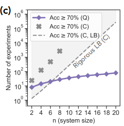
In addition to the theoretical work, we ran some proof-of-principle experiments on the Sycamore quantum processor. We started by implementing a QML algorithm to perform the first task. We fed an unknown quantum mixed state to the algorithm, then asked which of two observables of the state was larger. After training the neural network with simulation data, we found that the quantum learning agent needed exponentially fewer experiments to reach a prediction accuracy of 70% — equating to 10,000 times fewer measurements when the system size was 20 qubits. The total number of qubits used was 40 since two copies were stored at once.
 |
| Experimental comparison of QML vs. CML algorithms for predicting a quantum state’s observables. While the number of experiments needed to achieve 70% accuracy with a CML algorithm (“C” above) grows exponentially with the size of the quantum state n, the number of experiments the QML algorithm (“Q”) needs is only linear in n. The dashed line labeled “Rigorous LB (C)” represents the theoretical lower bound (LB) — the best possible performance — of a classical machine learning algorithm. |
<!–
 |
| Experimental comparison of QML vs. CML algorithms for predicting a quantum state’s observables. While the number of experiments needed to achieve 70% accuracy with a CML algorithm (“C” above) grows exponentially with the size of the quantum state n, the number of experiments the QML algorithm (“Q”) needs is only linear in n. The dashed line labeled “Rigorous LB (C)” represents the theoretical lower bound (LB) — the best possible performance — of a classical machine learning algorithm. |
–>
In a second experiment, relating to the task 3 above, we had the algorithm learn about the symmetry of an operator that evolves the quantum state of their qubits. In particular, if a quantum state might undergo evolution that is either totally random or random but also time-reversal symmetric, it can be difficult for a classical learner to tell the difference. In this task, the QML algorithm can separate the operators into two distinct categories, representing two different symmetry classes, while the CML algorithm fails outright. The QML algorithm was completely unsupervised, so this gives us hope that the approach could be used to discover new phenomena without needing to know the right answer beforehand.
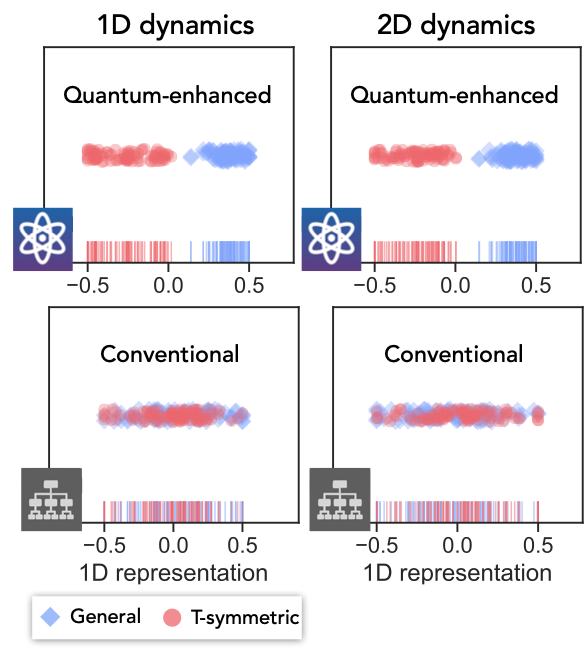 |
| Experimental comparison of QML vs. CML algorithms for predicting the symmetry class of an operator. While QML successfully separates the two symmetry classes, the CML fails to accomplish the task. |
Conclusion
This experimental work represents the first demonstrated exponential advantage in quantum machine learning. And, distinct from a computational advantage, when limiting the number of samples from the quantum state, this type of quantum learning advantage cannot be challenged, even by unlimited classical computing resources.
So far, the technique has only been used in a contrived, “proof-of-principle” experiment, where the quantum state is deliberately produced and the researchers pretend not to know what it is. To use these techniques to make quantum-enhanced measurements in a real experiment, we’ll first need to work on current quantum sensor technology and methods to faithfully transfer quantum states to a quantum computer. But the fact that today’s quantum computers can already process this information to squeeze out an exponential advantage in learning bodes well for the future of quantum machine learning.
Acknowledgements
We would like to thank our Quantum Science Communicator Katherine McCormick for writing this blog post. Images reprinted with permission from Huang et al., Science, Vol 376:1182 (2022).
Hello, would you mind sharing your strategies on how you label thousands of images for training for custom datasets you can’t find online?
submitted by /u/jchasinga
[visit reddit] [comments]
It may seem intuitive that AI and deep learning can speed up workflows — including novel drug discovery, a typically years-long and several-billion-dollar endeavor. But professors Artem Cherkasov and Olexandr Isayev were surprised to find that no recent academic papers provided a comprehensive, global research review of how deep learning and GPU-accelerated computing impact drug Read article >
The post Artem Cherkasov and Olexandr Isayev on Democratizing Drug Discovery With NVIDIA GPUs appeared first on NVIDIA Blog.


|
submitted by /u/joanna58 [visit reddit] [comments] |