Is it possible to make an AI-driven system that predicts gearbox failure on a simple $4 MCU? How to automatically build a compact model that does not require any additional compression? Can a non-data scientist implement such projects successfully?
I will answer all these questions in my new project.
In industry (e.g., wind power, automotive), gearboxes often operate under random speed variations. A condition monitoring system is expected to detect faults, broken tooth conditions and assess their severity using vibration signals collected under different speed profiles.
Modern cars have hundreds of thousands of details and systems where it is necessary to predict breakdowns, control the state of temperature, pressure, etc.As such, in the automotive industry, it is critically important to create and embed TinyML models that can perform right on the sensors and open up a set of technological advantages, such as:
- Internet independence
- No waste of energy and money on data transfer
- Advanced privacy and security
In my experiment I want to show how to easily create such a technology prototype to popularize the TinyML approach and use its incredible capabilities for the automotive industry.
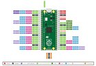
I used Neuton TinyML. I selected this solution since it is free to use and automatically creates tiny machine learning models deployable even on 8-bit MCUs. According to Neuton developers, you can create a compact model in one iteration without compression and Raspberry Pi Pico: The chip employs two ARM Cortex-M0 + cores, 133 megahertz, which are also paired with 256 kilobytes of RAM when mounted on the chip. The device supports up to 16 megabytes of off-chip flash storage, has a DMA controller, and includes two UARTs and two SPIs, as well as two I2C and one USB 1.1 controller. The device received 16 PWM channels and 30 GPIO needles, four of which are suitable for analog data input. And with a net $4 price tag.
https://preview.redd.it/vgsmg5wybcq81.png?width=740&format=png&auto=webp&s=4aea393b4286c63884ada3ce6085b7ce33f22afb
The goal of this tutorial is to demonstrate how you can easily build a compact ML model to solve a multi-class classification task to detect broken tooth conditions in the gearbox.
Gearbox Fault Diagnosis Dataset includes the vibration dataset recorded by using SpectraQuest’s Gearbox Fault Diagnostics Simulator.
Dataset has been recorded using 4 vibration sensors placed in four different directions and under variation of load from ‘0’ to ’90’ percent. Two different scenarios are included:1) Healthy condition 2) Broken tooth condition
There are 20 files in total, 10 for a healthy gearbox and 10 for a broken one. Each file corresponds to a given load from 0% to 90% in steps of 10%. You can find this dataset via the link in the comments!
https://preview.redd.it/hwvhote1ccq81.png?width=899&format=png&auto=webp&s=a6d96585131a51650f8df566367e535949f4b4e3
The experiment will be conducted on a $4 MCU, with no cloud computing carbon footprints 🙂
Step 1: Model training
For model training, I’ll use the free of charge platform, Neuton TinyML. Once the solution is created, proceed to the dataset uploading (keep in mind that the currently supported format is CSV only).
https://preview.redd.it/cmv3gnz3ccq81.png?width=740&format=png&auto=webp&s=66bb1d5de48702840a14061b882b7daa4e08de67
It’s time to select the target variable or the output you want for each prediction. In this case, we have class as Output Variable: ‘target’
https://preview.redd.it/sr98p5t6ccq81.png?width=740&format=png&auto=webp&s=682e9bcdc5a20a81ebc2981121b25ec183e415fd
Since the dataset is a vibration, we need to prepare the data before training the model. To do this, I select the setting Digital Signal Processing (DSP).
Digital Signal Processing (DSP) option enables automatic preprocessing and feature extraction for data from gyroscopes, accelerometers, magnetometers, electromyography (EMG), etc. Neuton will automatically transform raw data and extract additional features to create precise models for signal classification.
For this model, we use Accuracy as a metric (but you can experiment with all available metrics).
https://preview.redd.it/35c3kjwbccq81.png?width=740&format=png&auto=webp&s=6b23996a3b0ff9e8622516e0f7d91a5e6cc90d3f
While the model is being trained, you can check out Exploratory Data Analysis generated once the data processing is complete, you will get the full information with all the data!
The target metric for me was: Accuracy 0.921372 and the trained model had the following characteristics:
https://preview.redd.it/d49yakkeccq81.png?width=740&format=png&auto=webp&s=ef74542e06803ed6e930861a0acbdd659628b018
Number of coefficients = 397, File Size for Embedding = 2.52 Kb. That’s super cool! It is a really small model!Upon the model training completion, click on the Prediction tab, and then click on the Download button next to Model for Embedding to download the model library file that we are going to use for our device.
Step 2: Embedding on Raspberry Pico
Once you have downloaded the model files, it’s time to add our custom functions and actions. I am using Arduino IDE to program Raspberry Pico.
https://preview.redd.it/ojyzy6chccq81.png?width=1280&format=png&auto=webp&s=d0448c3900d41fb82d87a5088dc0d3d6a17e2eac
I used Ubuntu for this tutorial, but the same instructions should work for other Debian-based distributions such as Raspberry Pi OS.
- Open a terminal and use wget to download the official Pico setup script.
$ wget https://raw.githubusercontent.com/raspberrypi/pico-setup/master/pico_setup.sh
- In the same terminal modify the downloaded file so that it is executable.
$ chmod +x pico_setup.sh
-
Run pico_setup.sh to start the installation process. Enter your sudo password if prompted.
$ ./pico_setup.sh
-
Download the Arduino IDEand install it on your machine.
- Open a terminal and add your user to the group “dialout” and Log out or reboot your computer for the changes to take effect.
$ sudo usermod -a -G dialout “$USER”
-
Open the Arduino application and go to File >> Preferences. In the additional boards’ manager add this line and click OK.
https://github.com/earlephilhower/arduino-pico/releases/download/global/package_rp2040_index.json
https://preview.redd.it/abcx2u6kccq81.png?width=740&format=png&auto=webp&s=ef176b3d9dbfdde234cd3b3570edd45e39578c8f
-
Go to Tools >> Board >> Boards Manager. Type “pico” in the search boxand then install the Raspberry Pi Pico / RP2040 board. This will trigger another large download, approximately 300MB in size.
https://preview.redd.it/fccf3m1nccq81.png?width=740&format=png&auto=webp&s=ea795e0477be02c0035f7e1b1ae1191863f288d5
Note: Since we are going to make classification on the test dataset, we will use the CSV utility provided by Neuton to run inference on the data sent to the MCU via USB.
Here is our project directory,
user@desktop:~/Documents/Gearbox$ tree
. ├── application.c ├── application.h ├── checksum.c ├── checksum.h ├── Gearbox.ino ├── model │ └── model.h ├── neuton.c ├── neuton.h ├── parser.c ├── parser.h ├── protocol.h ├── StatFunctions.c ├── StatFunctions.h
3 directories, 14 files 1 directory, 13 files
Checksum, parser program files are for generating handshake with the CSV serial utility tool and sending column data to the Raspberry Pico for inference.
Understanding the code part in Gearbox.ino file, we set different callbacks for monitoring CPU, time, and memory usage used while inferencing.
void setup() {
Serial.begin(230400); while (!Serial);
pinMode(LED_RED, OUTPUT); pinMode(LED_BLUE, OUTPUT); pinMode(LED_GREEN, OUTPUT); digitalWrite(LED_RED, LOW); digitalWrite(LED_BLUE, LOW); digitalWrite(LED_GREEN, LOW);
callbacks.send_data = send_data; callbacks.on_dataset_sample = on_dataset_sample; callbacks.get_cpu_freq = get_cpu_freq; callbacks.get_time_report = get_time_report;
init_failed = app_init(&callbacks); }
The real magic happens here callbacks.on_dataset_sample=on_dataset_sample
static float* on_dataset_sample(float* inputs)
{ if (neuton_model_set_inputs(inputs) == 0) { uint16_t index; float* outputs; uint64_t start = micros(); if (neuton_model_run_inference(&index, &outputs) == 0) { uint64_t stop = micros(); uint64_t inference_time = stop – start; if (inference_time > max_time) max_time = inference_time; if (inference_time < min_time) min_time = inference_time; static uint64_t nInferences = 0; if (nInferences++ == 0) { avg_time = inference_time; } else { avg_time = (avg_time * nInferences + inference_time) / (nInferences + 1); } digitalWrite(LED_RED, LOW); digitalWrite(LED_BLUE, LOW); digitalWrite(LED_GREEN, LOW); switch (index) { /** Green Light means Gearbox Broken (10% load), Blue Light means Gearbox Broken (40% load), and Red Light means Gearbox Broken (90% load) based upon the CSV test dataset received via Serial. **/ case 0: //Serial.println(“0: Healthy 10% load”); break; case 1: //Serial.println(“1: Broken 10% load”); digitalWrite(LED_GREEN, HIGH); break; case 2: //Serial.println(“2: Healthy 40% load”); break; case 3: //Serial.println(“3: Broken 40% load”); digitalWrite(LED_BLUE, HIGH); break; case 4: //Serial.println(“4: Healthy 90% load”); break; case 5: //Serial.println(“5: Broken 90% load”); digitalWrite(LED_RED, HIGH); break; default: break; } return outputs; } } return NULL; }
Once the input variables are ready, neuton_model_run_inference(&index, &outputs) is called which runs inference and returns outputs.
Installing CSV dataset Uploading Utility (Currently works on Linux and macOS only)
# For Ubuntu
$ sudo apt install libuv1-dev gengetopt
For macOS
$ brew install libuv gengetopt
$ git clone https://github.com/Neuton-tinyML/dataset-uploader.git
$ cd dataset-uploader
- Run make to build the binaries,
$ make
Once it’s done, you can try running the help command, it’s should be similar to shown below
user@desktop:~/dataset-uploader$ ./uploader -h
Usage: uploader [OPTION]… Tool for upload CSV file MCU -h, –help Print help and exit -V, –version Print version and exit -i, –interface=STRING interface (possible values=”udp”, “serial” default=serial’) -d, –dataset=STRING Dataset file (default=
./dataset.csv’) -l, –listen-port=INT Listen port (default=50000′) -p, –send-port=INT Send port (default=
50005′) -s, –serial-port=STRING Serial port device (default=/dev/ttyACM0′) -b, –baud-rate=INT Baud rate (possible values=”9600″, “115200”, “230400” default=
230400′) –pause=INT Pause before start (default=`0′)
Step 3: Running inference on Raspberry Pico
Upload the program on the Raspberry Pico,
https://preview.redd.it/rib4jtg3dcq81.png?width=740&format=png&auto=webp&s=2bf5d32b6865c52f297cd160da305fc09df49a38
Once uploaded and running, open a new terminal and run this command:
$ ./uploader -s /dev/ttyACM0 -b 230400 -d /home/vil/Desktop/Gearbox_10_40_90_test.csv
https://preview.redd.it/pq2zsyl6dcq81.png?width=740&format=png&auto=webp&s=225f05ab4420f52b4f546f6596e8c85963aa8942
The inference has started running, once it is completed for the whole CSV dataset it will print a full summary.
>> Request performace report
Resource report: CPU freq: 125000000 Flash usage: 2884 RAM usage total: 2715 RAM usage: 2715 UART buffer: 42
Performance report: Sample calc time, avg: 44172.0 us Sample calc time, min: 43721.0 us Sample calc time, max: 44571.0 us
I tried to build the same model with TensorFlow and TensorFlow Lite as well. My model built with Neuton TinyML turned out to be 4.3% better in terms of Accuracy and 15.3 times smaller in terms of model size than the one built with TF Lite. Speaking of the number of coefficients, TensorFlow’s model has,9, 330 coefficients, while Neuton’s model has only 397 coefficients (which is 23.5 times smallerthan TF!).
The resultant model footprint and inference time are as follows:
https://preview.redd.it/i1yyxl5mdcq81.png?width=740&format=png&auto=webp&s=53996adaa83ca6a1d243a88ebba5cc145ee5e7ae
This tutorial vividly demonstrates the huge impact that TinyML technologies can provide on the automotive industry. You can have literally zero data science knowledge but still rapidly build super compact ML models to effectively solve practical challenges. And the best part, it’s all possible by using an absolutely free solution and a super cheap MCU!

 Learn about the H100 CNX, an innovative new hardware accelerator for GPU-accelerated I/O intensive workloads.
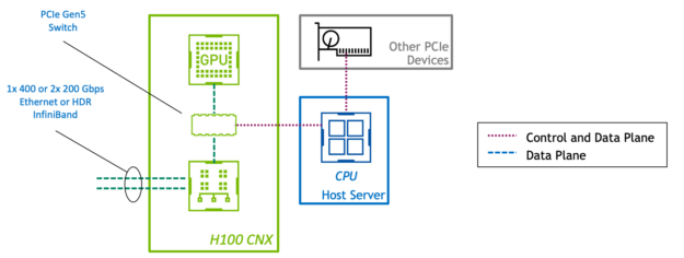
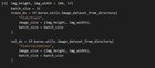
High training accuracy and low validation accuracy")
 MarshallAI is using NVIDIA GPU accelerated technologies to help cities improve their traffic management, reduce carbon emissions, and save drivers time.
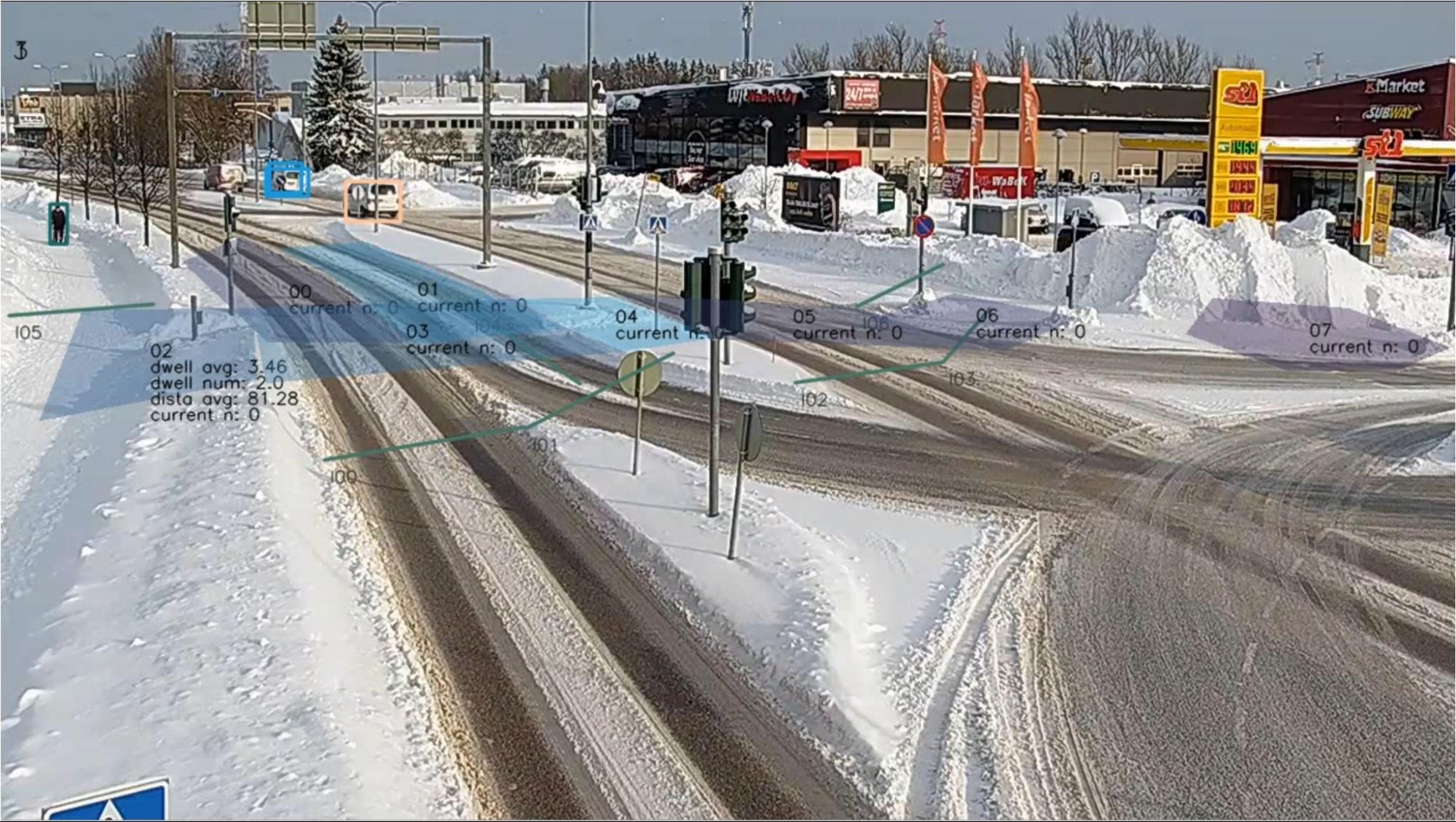
