Categories
Misc

Choosing a Server for Deep Learning Inference

Learn about the characteristics of inference workloads and systems features needed to run them, particularly at the edge.

Inference is an important part of the machine learning lifecycle and occurs after you have trained your model. It is when a business realizes value from their AI investment. Common applications of AI include image classification (“this is an image of a tumor”), recommendation (“here is a movie you will like”), transcription of speech audio into text, and decision (“turn the car to the left”). 

Systems for deep learning training require a lot of computing capabilities, but after an AI model has been trained, fewer resources are needed to run it in production. The most important factors in determining the system requirements for inference workloads are the model being run and the deployment location. This post discusses these areas, with a particular focus on AI inference at the edge.

AI model inference requirements

For help with determining the optimal inference deployment configuration, a tool like NVIDIA Triton Model Analyzer makes recommendations based on the specific AI models that are running. An inference compiler like NVIDIA TensorRT can reduce the resource requirements for inference by optimizing the model to run with the highest throughput and lowest latency while preserving accuracy.

Even with these optimizations, GPUs are still critical to achieving the business service level objectives SLAs and requirements for inference workloads. Results from the MLPerf 2.0 Inference benchmark demonstrate that NVIDIA GPUs are more than 100x faster than CPU-only systems. GPUs can also provide the low latency required for workloads that need a real-time response. 

Deployment locations of inference workloads

AI inference workloads can be found both in the data center as well as at the edge. Examples of inference workloads running in a data center include recommender systems and natural language processing. 

There is great variety in the way these workloads can be run. For example, many different models can be served simultaneously from the same servers, and there can be hundreds, thousands, or even tens of thousands of concurrent inference requests in flight. In addition, data center servers often run other workloads besides AI inference. 

There is no “one size fits all” solution when it comes to system design for data center inference.

Inference applications running at edge locations represent an important and growing class of workloads. Edge computing is driven by the requirement for low-latency, real-time results as well as the desire to reduce data transit for both cost and security reasons. Edge systems run in locations physically close to where data is collected or processed, in settings such as retail stores, factory floors, and cell phone base stations.

As compared with data center inference, system requirements for AI inference at the edge are easier to articulate, because these systems are usually designed to focus on a narrow range of inference workloads.

Edge inference typically involves either a camera or other sensor gathering data that must be acted upon. An example of this could be sensor-equipped video cameras in chemical plants being used to detect corrosion in pipes and alert staff before any damage is done.

Edge inference system requirements

Servers for AI training must be designed to process large amounts of historical data to learn the right values for model parameters. By contrast, servers for edge inference are required to process streaming data being gathered in real time at the edge location, which is smaller in volume.

As a result, system memory doesn’t need to be as large, and the number of CPU cores can be lower. The network adapter doesn’t need as high bandwidth and the local storage on the server can be smaller as it’s not caching any training data sets.

However, both the networking and storage should be configured to enable the lowest latency, as the ability to respond as quickly as possible is critical.

Resource AI training in the data center AI inferencing at the edge
CPU Fastest CPUs with high core count Lower-power CPUs
GPU Fastest GPUs with most memory, more GPUs per system Lower-power GPU, or larger GPU with MIG, one or two GPUs per system
Memory Large memory size Average memory size
Storage High bandwidth NVMe flash drive, one per CPU Average bandwidth, lowest-latency NVMe flash drive, one per system
Network Highest bandwidth network adapter, Ethernet or InfiniBand, one per GPU pair Average bandwidth network adapter, Ethernet, one per system
PCIe System Devices balanced across PCIe topology; PCIe switch for multi-GPU, multi-NIC deployments Devices balanced across PCIe topology; PCIe switch not required
Table 1. Resource recommendations for data center training and edge inferencing

Edge systems are by definition deployed outside traditional data centers, often in remote locations. The environment is often constrained in terms of space and power. These constraints can be met by using smaller systems in conjunction with low-powered GPUs, such as the NVIDIA A2. 

If the inference workload is more demanding, and power budgets allow it, then a larger GPU, such as the NVIDIA A30 or NVIDIA A100, can be used. The Multi-Instance GPU (MIG) feature enables these GPUs to service multiple inference streams simultaneously so that the system overall can provide highly efficient performance.

Other factors for edge inference

Beyond system requirements, there are other factors to consider that are unique to the edge.

Host security

Security is a critical aspect of edge systems. Data centers by their nature can provide a level of physical control as well as centralized management that can prevent or mitigate attempts to steal information or take control of servers.

Edge systems must be designed with the assumption that their deployment locations are not physically secured, and that they cannot benefit from as many of the access control mechanisms found in data center IT management systems.

Trusted Platform Module (TPM) is one technology that can help greatly with host security. Configured appropriately, a TPM can ensure that the system can only boot with firmware and software that has been digitally signed and unaltered. Additional security checks such as signed containers ensure that applications haven’t been tampered with, and disk volumes can be encrypted with keys that are securely stored in the TPM.

Encryption

Another important consideration is the encryption of all network traffic to and from the edge system. Signed network adapters with encryption acceleration hardware, as found in NVIDIA ConnectX products, ensure that this protection doesn’t come at the expense of a reduction in data transfer rates.

Ruggedized systems

For certain use cases, such as on a factory floor for automation control or in an enclosure next to a telecommunications antenna tower, edge systems must perform well under potentially harsh conditions, such as elevated temperatures, large shock and vibration, and dust.

Ruggedized servers designed for these purposes are increasingly available with GPUs, thus allowing even these extreme use cases to benefit from greatly higher performance.

Choose an end-to-end platform for inference

NVIDIA has extended the NVIDIA-Certified Systems program to include categories for edge deployments that run outside a traditional data center. The design criteria for these systems include all of the following:

  • NVIDIA GPUs
  • CPU, memory, and network configurations that provide optimal performance
  • Security and remote management capabilities

The Qualified System Catalog has a list of NVIDIA-Certified systems from NVIDIA partners. The list can be filtered by category of system, including the following that are ideal for inference workloads: 

  • Data Center servers are validated for performance and scale-out capabilities on a variety of data science workloads and are ideal for data center inference.
  • Enterprise Edge systems are designed to be deployed in controlled environments, such as the back office of a retail store. Systems in this category are tested in data center-like environments.
  • Industrial Edge systems are designed for industrial or rugged environments, such as a factory floor or cell phone tower base station. Systems that achieve this certification must pass all tests while running within the environment for which the system was designed, such as elevated temperature environments outside of the typical data center range.

In addition to certifying systems for the edge, NVIDIA has also developed enterprise software to run and manage inference workloads.

NVIDIA Triton Inference Server streamlines AI inference by enabling teams to deploy, run, and scale trained AI models from any framework on any GPU- or CPU-based infrastructure. It helps you deliver high-performance inference across cloud, on-premises, edge, and embedded devices. 

NVIDIA AI Enterprise is an end-to-end, cloud-native suite of AI and data analytics software, optimized so every organization can be good at AI, certified to deploy in both data center and edge locations. It includes global enterprise support so that AI projects stay on track.

NVIDIA Fleet Command is a cloud service that centrally connects systems at edge locations to securely deploy, manage, and scale AI applications from one dashboard. It’s turnkey with layers of security protocols and can be fully functional in hours.

By choosing an end-to-end platform consisting of certified systems and infrastructure software, you can kick-start your AI production deployments and have inference applications deployed and running much more quickly than trying to assemble a solution from individual components.

Learn more about the NVIDIA AI Inference platform 

There’s a lot more involved when it comes to deep learning inference. The NVIDIA AI Inference Platform Technical Overview has an in-depth discussion of this topic, including a view of the end-to-end deep learning workflow, the details of taking AI-enabled applications from prototype to production deployments, and software frameworks for building and running AI inference applications.

Sign up for Edge AI News to stay up to date with the latest trends, customer use cases, and technical walkthroughs.
Categories
Misc

Getting Started with NVIDIA Instant NeRFs

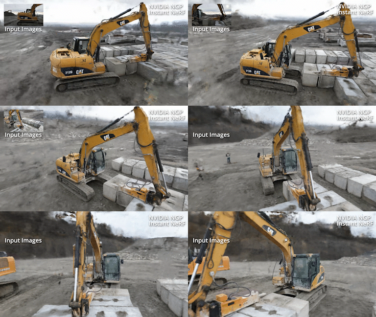
A neural radiance field rendering an image of an excavator in a 3d sceneJohnathan Stephens provides a walkthrough of how he started using Instant NeRF.A neural radiance field rendering an image of an excavator in a 3d scene
The new NVIDIA NGP Instant NeRF is a great introduction to getting started with neural radiance fields. In as little as an hour, you can compile the codebase, prepare your images, and train your first NeRF. Unlike other NeRF implementations, Instant NeRF only takes a few minutes to train a great-looking visual.

In my hands-on video (embedded), I walk you through the ins and outs of making your first NeRF. I cover a couple of key tips to help you compile the codebase and explain how to capture good input imagery. I walk through the GUI interface and explain how to optimize your scene parameters. Finally, I show you have to create an animation from your scene.

Video 1. Hands-on with NVIDIA Instant NeRFs

Compiling the codebase

The codebase is straightforward to compile for experienced programmers and data scientists. Beginners can easily follow the detailed instructions provided in bycloudai’s fork from the main GitHub repository. Here are a few additional tips that helped with the installation process:

Capturing imagery for Instant NeRF

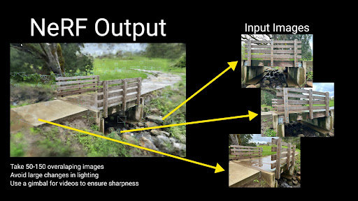
The pipeline accepts both photo and video input for Instant NeRF generation. The first step in the Instant NeRF generation pipeline uses COLMAP to determine camera positions. Due to this fact, you must follow basic principles of photogrammetry with respect to overlapping and sharp imagery. The video shows you example imagery from an ideal capture.

Photos with callouts: Avoid changes in lighting, use a gimbal to ensure sharpness, and take 50-150 overlapping images.
Figure 1. A few tips on input images to improve the quality of the NeRF output

Launching the GUI and training your first NeRF

When the images’ positions are prepared for your first Instant NeRF, launch the graphical user interface through Anaconda using the included Testbed.exe file compiled from the codebase. The NeRF automatically starts training your NeRF.

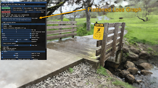
You will find a majority of visual quality gained in the first 30 seconds; however, your NeRF will continue to improve over several minutes. The loss graph in the GUI eventually flattens out and you can stop the training to improve your viewer’s framerate.

Screenshot with a callout indicating where to find the Flattened loss graph within the GUI.
Figure 2. Snapshot of the GUI within the Instant NeRF software highlights the flattened loss graph

The GUI includes many visualization options, including controls over the camera and debug visualizations. I cover several different options in the GUI in the hands-on demo video.

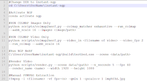
Tip: save your commonly used command-line prompts in Notepad for future reference.

Figure 3- Share your commonly used command prompts in a notepad for ease of use later on.
Figure 3. Command-line prompts within the software

Creating an animation

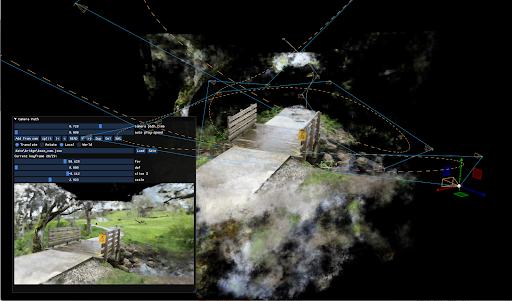
NVIDIA provides an easy-to-use camera path editor with the GUI. To add keyframes, navigate through the scene and choose Add from Cam. The GUI generates a camera trajectory with Bézier curves. To preview your animation, choose Read. When you are happy with the animation, save your camera path and render a full-quality video with the render script in your scripts folder.

Screenshot of the static images rendering into a 3D scene.
Figure 4. Instant NeRF renders the static images into a 3D scene

Conclusion

One large benefit that I’ve found with Instant NeRFs is that I capture the entire background as part of the scene. Using photogrammetry, I lose the context of the object’s surroundings. This fact excites me as it unlocks a whole new world of potential for capturing and visualizing the world in new ways.

I found that experimenting with NVIDIA Instant NeRFs has been a great introduction to emerging technology. The speed at which I am able to produce results means that I can quickly learn about what works for image capturing. I hope that this walkthrough benefits you as you start your own journey to explore the power and fun of NeRFs.

Stay tuned

Now that you know how to capture a set of images and transform them into a 3D scene, we suggest you get practicing. NVIDIA will be hosting a competition for the chance to win the newest GPU to hit the market, an NVIDIA RTX 3090 Ti. Follow NVIDIA on Twitter and LinkedIn to stay in touch with the competition announcement in late May.

Categories
Offsites

Challenges in Multi-objective Optimization for Automatic Wireless Network Planning

Economics, combinatorics, physics, and signal processing conspire to make it difficult to design, build, and operate high-quality, cost-effective wireless networks. The radio transceivers that communicate with our mobile phones, the equipment that supports them (such as power and wired networking), and the physical space they occupy are all expensive, so it’s important to be judicious in choosing sites for new transceivers. Even when the set of available sites is limited, there are exponentially many possible networks that can be built. For example, given only 50 sites, there are 250 (over a million billion) possibilities!

Further complicating things, for every location where service is needed, one must know which transceiver provides the strongest signal and how strong it is. However, the physical characteristics of radio propagation in an environment containing buildings, hills, foliage, and other clutter are incredibly complex, so accurate predictions require sophisticated, computationally-intensive models. Building all possible sites would yield the best coverage and capacity, but even if this were not prohibitively expensive, it would create unacceptable interference among nearby transceivers. Balancing these trade-offs is a core mathematical difficulty.

The goal of wireless network planning is to decide where to place new transceivers to maximize coverage and capacity while minimizing cost and interference. Building an automatic network planning system (a.k.a., auto-planner) that quickly solves national-scale problems at fine-grained resolution without compromising solution quality has been among the most important and difficult open challenges in telecom research for decades.

To address these issues, we are piloting network planning tools built using detailed geometric models derived from high-resolution geographic data, that feed into radio propagation models powered by distributed computing. This system provides fast, high-accuracy predictions of signal strength. Our optimization algorithms then intelligently sift through the exponential space of possible networks to output a small menu of candidate networks that each achieve different desirable trade-offs among cost, coverage, and interference, while ensuring enough capacity to meet demand.

Example auto-planning project in Charlotte, NC. Blue dots denote selected candidate sites. The heat map indicates signal strength from the propagation engine. The inset emphasizes the non-isotropic path loss in downtown.

<!–

Example auto-planning project in Charlotte, NC. Blue dots denote selected candidate sites. The heat map indicates signal strength from the propagation engine. The inset emphasizes the non-isotropic path loss in downtown.

–>

Radio Propagation
The propagation of radio waves near Earth’s surface is complicated. Like ripples in a pond, they decay with distance traveled, but they can also penetrate, bounce off, or bend around obstacles, further weakening the signal. Computing radio wave attenuation across a real-world landscape (called path loss) is a hybrid process combining traditional physics-based calculations with learned corrections accounting for obstruction, diffraction, reflection, and scattering of the signal by clutter (e.g., trees and buildings).

We have developed a radio propagation modeling engine that leverages the same high-res geodata that powers Google Earth, Maps and Street View to map the 3D distribution of vegetation and buildings. While accounting for signal origin, frequency, broadcast strength, etc., we train signal correction models using extensive real-world measurements, which account for diverse propagation environments — from flat to hilly terrain and from dense urban to sparse rural areas.

While such hybrid approaches are common, using detailed geodata enables accurate path loss predictions below one-meter resolution. Our propagation engine provides fast point-to-point path loss calculations and scales massively via distributed computation. For instance, computing coverage for 25,000 transceivers scattered across the continental United States can be done at 4 meter resolution in only 1.5 hours, using 1000 CPU cores.

Photorealistic 3D model in Google Earth (top-left) and corresponding clutter height model (top-right). Path profile through buildings and trees from a source to destination in the clutter model (bottom). Gray denotes buildings and green denotes trees.

Auto-Planning Inputs
Once accurate coverage estimates are available, we can use them to optimize network planning, for example, deciding where to place hundreds of new sites to maximize network quality. The auto-planning solver addresses large-scale combinatorial optimization problems such as these, using a fast, robust, scalable approach.

Formally, an auto-planning input instance contains a set of demand points (usually a square grid) where service is to be provided, a set of candidate transceiver sites, predicted signal strengths from candidate sites to demand points (supplied by the propagation model), and a cost budget. Each demand point includes a demand quantity (e.g., estimated from the population of wireless users), and each site includes a cost and capacity. Signal strengths below some threshold are omitted. Finally, the input may include an overall cost budget.

Data Summarization for Large Instances
Auto-planning inputs can be huge, not just because of the number of candidate sites (tens of thousands), and demand points (billions), but also because it requires signal strengths to all demand points from all nearby candidate sites. Simple downsampling is insufficient because population density may vary widely over a given region. Therefore, we apply methods like priority sampling to shrink the data. This technique produces a low-variance, unbiased estimate of the original data, preserving an accurate view of the network traffic and interference statistics, and shrinking the input data enough that a city-size instance fits into memory on one machine.

Multi-objective Optimization via Local Search
Combinatorial optimization remains a difficult task, so we created a domain-specific local search algorithm to optimize network quality. The local search algorithmic paradigm is widely applied to address computationally-hard optimization problems. Such algorithms move from one solution to another through a search space of candidate solutions by applying small local changes, stopping at a time limit or when the solution is locally optimal. To evaluate the quality of a candidate network, we combine the different objective functions into a single one, as described in the following section.

The number of local steps to reach a local optimum, number of candidate moves we evaluate per step, and time to evaluate each candidate can all be large when dealing with realistic networks. To achieve a high-quality algorithm that finishes within hours (rather than days), we must address each of these components. Fast candidate evaluation benefits greatly from dynamic data structures that maintain the mapping between each demand point and the site in the candidate solution that provides the strongest signal to it. We update this “strongest-signal” map efficiently as the candidate solution evolves during local search. The following observations help limit both the number of steps to convergence and evaluations per step.

Bipartite graph representing candidate sites (left) and demand points (right). Selected sites are circled in red, and each demand point is assigned to its strongest available connection. The topmost demand point has no service because the only site that can reach it was not selected. The third and fourth demand points from the top may have high interference if the signal strengths attached to their gray edges are only slightly lower than the ones on their red edges. The bottommost site has high congestion because many demand points get their service from that site, possibly exceeding its capacity.

Selecting two nearby sites is usually not ideal because they interfere. Our algorithm explicitly forbids such pairs of sites, thereby steering the search toward better solutions while greatly reducing the number of moves considered per step. We identify pairs of forbidden sites based on the demand points they cover, as measured by the weighted Jaccard index. This captures their functional proximity much better than simple geographic distance does, especially in urban or hilly areas where radio propagation is highly non-isotropic.

Breaking the local search into epochs also helps. The first epoch mostly adds sites to increase the coverage area while avoiding forbidden pairs. As we approach the cost budget, we begin a second epoch that includes swap moves between forbidden pairs to fine-tune the interference. This restriction limits the number of candidate moves per step, while focusing on those that improve interference with less change to coverage.

Three candidate local search moves. Red circles indicate selected sites and the orange edge indicates a forbidden pair.

Outputting a Diverse Set of Good Solutions
As mentioned before, auto-planning must balance three competing objectives: maximizing coverage, while minimizing interference and capacity violations, subject to a cost budget. There is no single correct tradeoff, so our algorithm delegates the final decision to the user by providing a small menu of candidate networks with different emphases. We apply a multiplier to each objective and optimize the sum. Raising the multiplier for a component guides the algorithm to emphasize it. We perform grid search over multipliers and budgets, generating a large number of solutions, filter out any that are worse than another solution along all four components (including cost), and finally select a small subset that represent different tradeoffs.

Menu of candidate solutions, one per row, displaying metrics. Clicking on a solution turns the selected sites pink and displays a plot of the interference distribution across covered area and demand. Sites not selected are blue.

Conclusion
We described our efforts to address the most vexing challenges facing telecom network operators. Using combinatorial optimization in concert with geospatial and radio propagation modeling, we built a scalable auto-planner for wireless telecommunication networks. We are actively exploring how to expand these capabilities to best meet the needs of our customers. Stay tuned!

For questions and other inquiries, please reach out to wireless-network-interest@google.com.

Acknowledgements
These technological advances were enabled by the tireless work of our collaborators: Aaron Archer, Serge Barbosa Da Torre, Imad Fattouch, Danny Liberty, Pishoy Maksy, Zifei Tong, and Mat Varghese. Special thanks to Corinna Cortes, Mazin Gilbert, Rob Katcher, Michael Purdy, Bea Sebastian, Dave Vadasz, Josh Williams, and Aaron Yonas, along with Serge and especially Aaron Archer for their assistance with this blog post.

Categories
Misc

Urban Jungle: AI-Generated Endangered Species Mix With Times Square’s Nightlife

Bengal tigers, red pandas and mountain gorillas are among the world’s most familiar endangered species, but tens of thousands of others — like the Karpathos frog, the Perote deer mouse or the Mekong giant catfish — are largely unknown. Typically perceived as lacking star quality, these species are now roaming massive billboards in one of Read article >

The post Urban Jungle: AI-Generated Endangered Species Mix With Times Square’s Nightlife appeared first on NVIDIA Blog.

Categories
Misc

Colab is slow?

I’m running cifar100 on resnet50 modal. On my local machine, I have a 1050ti(and on colab, I do have the GPU on)

I get half the train time per epoch on my local machine than via colab even though colab is running on a k80. is this normal

This is my code: https://colab.research.google.com/drive/1HU-vPLy0VLMVe7JebHJjeD4Mmw6MgTVl?usp=sharing

(its just used for testing)

​

submitted by /u/Mayfieldmobster
[visit reddit] [comments]

Categories
Misc

GFN Thursday Gets Groovy As ‘Evil Dead: The Game’ Marks 1,300 Games on GeForce NOW

Good. Bad. You’re the Guy With the Gun this GFN Thursday. Get ready for some horrifyingly good fun with Evil Dead: The Game streaming on GeForce NOW tomorrow at release. It’s the 1,300th game to join GeForce NOW, joining on Friday the 13th. And it’s part of eight total games joining the GeForce NOW library Read article >

The post GFN Thursday Gets Groovy As ‘Evil Dead: The Game’ Marks 1,300 Games on GeForce NOW appeared first on NVIDIA Blog.

Categories
Misc

Question about tensorflow models

I’m currently an intern trying to wrap Face-api.js as a component, my problem is – and I think I know too little about to fully understand – the models.
I was wondering if there are other ways to save and load (already feeded) models, other than using script tags. I need to be looking into it to get a better performance rate, but I honestly don’t know if this is even a possibility.

submitted by /u/KawaiiFromOuterSpace
[visit reddit] [comments]

Categories
Misc

NVIDIA Transitioning To Official, Open-Source Linux GPU Kernel Driver

NVIDIA Transitioning To Official, Open-Source Linux GPU Kernel Driver submitted by /u/nikniuq
[visit reddit] [comments]
Categories
Misc

Tensorflow performing worst in better hardware

I am migrating from a laptop with a RTX 3080 mobile to a desktop with a RTX3080 Ti. I am using the Tensorflow Docker image from the NGC Catalog (tensorflow:22.03-tf2-py3) in both instances and the same code/dataset. The laptop was running Pop OS 20.04 LTS and the desktop Ubuntu 20.04 LTS, basically the same setup.

The laptop took about 2 seconds per epoch (can’t re test again because I have to turn in the device, but epoch time is stored in the Jupiter notebook) while the desktop (with better a GPU) takes between 4 to 5 seconds. I already re-installed drivers and the whole docker engine with no luck. Currently while checking nvidia-smi gpu usage is only about 30%.

Does anyone has encountered a problem like this? Thanks.

submitted by /u/CESARIUX2596
[visit reddit] [comments]

Categories
Misc

Accelerating AI Inference Workloads with NVIDIA A30 GPU

A30 enables researchers, engineers, and data scientists to deliver real-world results and deploy solutions into production at scale.

NVIDIA A30 GPU is built on the latest NVIDIA Ampere Architecture to accelerate diverse workloads like AI inference at scale, enterprise training, and HPC applications for mainstream servers in data centers. The A30 PCIe card combines the third-generation Tensor Cores with large HBM2 memory (24 GB) and fast GPU memory bandwidth (933 GB/s) in a low-power envelope (maximum 165 W).

A30 supports a broad range of math precisions:

  • double-precision (FP64)
  • single-precision (FP32)
  • half-precision (FP16)
  • Brain Float 16 (BF16)
  • Integer (INT8)

It also supports innovations such as Tensor Float 32 (TF32) and Tensor Core FP64, providing a single accelerator to speed up every workload.

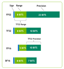
Figure 1 shows TF32, which has the range of FP32 and precision of FP16. TF32 is the default option in PyTorch, TensorFlow, and MXNet, so no code change is needed to achieve speedup over the last-generation NVIDIA Volta Architecture.

Different precisions and their representations in bits: FP32 has 1 bit for sign, 8 bits for range, and 23 bits for precision. TF32 has 1 bit for sign, 8 bits for range, and 10 bits for precision. FP16 has 1 bit for sign, 5 bits for range, and 10 bits for precision. BF16 has 1 bit for sign, 8 bits for range, and 7 bits for precision.
Figure 1. TF32 and other precisions in bit numbers

Another important feature of A30 is Multi-Instance GPU (MIG) capability. MIG can maximize the GPU utilization across big to small workloads and ensure quality of service (QoS). A single A30 can be partitioned to up to four MIG instances to run four applications simultaneously, each fully isolated with its own streaming multiprocessors (SMs), memory, L2 cache, DRAM bandwidth, and decoder. For more information, see Supported MIG Profiles.

For interconnection, A30 supports both PCIe Gen4 (64 GB/s) and the high-speed third-generation NVLink (maximum 200 GB/s). Each A30 can support one NVLink bridge connection with a single adjacent A30 card. Wherever an adjacent pair of A30 cards exists in the server, the pair should be connected by the NVLink bridge that spans two PCIe slots for best bridging performance and balanced bridge topology.

​ NVIDIA T4 NVIDIA A30
Design Small Footprint Data Center & Edge Inference AI Inference & Mainstream Compute
Form Factor x16 PCIe Gen3
1 slot LP
x16 PCIe Gen4
2 Slot FHFL
1 NVLink bridge
Memory 16GB GDDR6 24GB HBM2
Memory Bandwidth​ 320 GB/s 933 GB/s
Multi-Instance GPU   Up to 4
Media Acceleration 1 Video Encoder 2 Video Decoder 1 JPEG Decoder 4 Video Decoder
Fast FP64 No Yes
Ray Tracing Yes No
Power ​ 70W 165W
Table 1. Summary of the features of A30 and T4

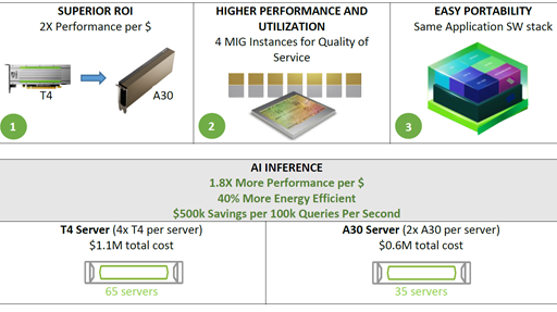
In addition to the hardware benefits summarized in Table 1, A30 ​​can achieve higher performance per dollar compared to the T4 GPU. A30 also supports end-to-end software stack solutions:

  • Libraries
  • GPU-accelerated deep learning frameworks like PyTorch, TensorFlow, and MXNet
  • Optimized deep learning models
  • Over 2,000 HPC and AI applications, which can be obtained from NGC containers

Performance analysis

To analyze the performance improvement of A30 over T4, and CPUs, we benchmarked six models from MLPerf Inference v1.1 with the datasets:

  • ResNet-50 v1.5 (ImageNet)
  • SSD-Large ResNet-34 (COCO)
  • 3D-Unet (BraTS 2019)
  • DLRM (1TB Click Logs, offline scenario)
  • BERT (SQuAD v1.1, seq-len: 384)
  • RNN-T (LibriSpeech)

The MLPerf benchmark suite covers a broad range of inference use cases, from image classification and object detection to recommenders, and natural language processing (NLP).

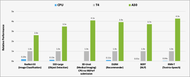
Figure 2 shows the results of the performance comparison of A30 with T4 and CPU on AI inference workloads.A30 is around 300x faster than a CPU for BERT inference.

Compared to T4, A30 delivers around 3-4x performance speedup for inference using the six models. The performance speedup is due to A30 larger memory size. This enables larger batch size for the models and faster GPU memory bandwidth (almost 3x T4), which can send the data to compute cores in a much shorter time.

[ALT: Bar chart uses T4 as a baseline. A30 achieves 2.6x perf on ResNet-50 compared to 0.20x on CPU, 3.5X perf on SSD-Large compared to 0.13x, 4.1x perf on 3D-UNet, 3.9x perf compared to 0.11x on DLRM, 3.7x perf on BERT compared to 0.01x, and 4.3x perf on RNN-T compared to 0.04x.
Figure 2. Performance comparison of A30 over T4 and CPU using MLPerf.
CPU: 8380H (no submission on 3D-Unet)

In addition to AI inference, A30 can rapidly pre-train AI models such as BERT Large with TF32, as well as accelerate HPC applications using FP64 Tensor Cores. A30 Tensor Cores with TF32 provide up to 10x higher performance over the T4 without requiring any changes in your code. They also provide an additional 2x boost with automatic mixed precision, delivering a combined 20x throughput increase.

Hardware decoders

While building a video analytics or video processing pipeline, there are several operations that must be considered:

  • Compute requirements for your model or preprocessing steps. This comes down to the Tensor Cores, GPU DRAM, and other hardware components that accelerate the models or frame preprocessing kernels.
  • Video stream encoding before transmission. This is done to minimize the bandwidth required on the network. To accelerate this workload, make use of NVIDIA hardware decoders.
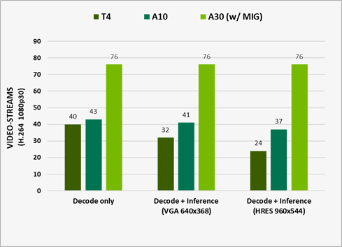
Bar chart of the total throughput of combined video decoding operations and model inference. A30 can process up to 76 1080p streams.
Figure 3. The number of streams being processed on different GPUs

Measured performance with DeepStream 5.1. It represents e2e performance with video capture and decode, preprocessing, batching, inference, and post-processing. Output rendering was turned off for optimal perf running ResNet10, ResNet18, and ResNet50 networks for inference on H.264 1080p30 video-streams.

A30 is designed to accelerate intelligent video analysis (IVA) by providing four video decoders, one JPEG decoder, and one optical flow decoder.

To make use of these decoders along with the compute resources for analyzing videos, use the NVIDIA DeepStream SDK, which delivers a complete streaming analytics toolkit for AI-based, multisensor processing, video, audio, and image understanding. For more information, see TAO Toolkit Integration with DeepStream or Building a Real-time Redaction App Using NVIDIA DeepStream, Part 1: Training.

What’s next?

Representing the most powerful end-to-end AI and HPC platform for data centers, A30 enables researchers, engineers, and data scientists to deliver real-world results and deploy solutions into production at scale. For more information, see the NVIDIA A30 Tensor Core GPU datasheet and NVIDIA A30 GPU Accelerator product brief.