If you want to ride the next big wave in AI, grab a transformer. They’re not the shape-shifting toy robots on TV or the trash-can-sized tubs on telephone poles. So, What’s a Transformer Model? A transformer model is a neural network that learns context and thus meaning by tracking relationships in sequential data like the Read article >
When the first instant photo was taken 75 years ago with a Polaroid camera, it was groundbreaking to rapidly capture the 3D world in a realistic 2D image. Today, AI researchers are working on the opposite: turning a collection of still images into a digital 3D scene in a matter of seconds. Known as inverse Read article >
NVIDIA announced a number of new tools for game developers at this year’s GDC to help you save time, more easily integrate RTX, and simplify the creation of virtual worlds.
This week at GDC, NVIDIA announced a number of new tools for game developers to help save time, more easily integrate NVIDIA RTX, and streamline the creation of virtual worlds. Watch this overview of three exciting new tools now available.
Figure 1. NVIDIA announces a number of new tools for game developers to help save time, more easily integrate NVIDIA RTX, and streamline the creation of virtual worlds.
Simplify integration with the new NVIDIA Streamline
Since NVIDIA Deep Learning Super Sampling (DLSS) launched in 2019, a variety of super-resolution technologies have shipped from both hardware vendors and engine providers. To support these various technologies, game developers have had to integrate multiple SDKs, often with varying integration points and compatibility.
Today NVIDIA is releasing Streamline, an open-source cross-IHV framework that aims to simplify integration of multiple super-resolution technologies and other graphics effects in games and applications.
Streamline offers a single integration with a plug-and-play framework. It sits between the game and render API, and abstracts the SDK-specific API calls into an easy-to-use Streamline framework. Instead of manually integrating each SDK, developers simply identify which resources (motion vectors, depth, etc) are required for the target super-resolution plug-ins and then set where they want the plug-ins to run in their graphics pipeline. The framework is also extensible beyond super-resolution SDKs, with developers able to add NVIDIA Real-time Denoisers (NRD) to their games via Streamline. Making multiple technologies easier for developers to integrate, Streamline benefits gamers with more technologies in more games.
Figure 2. Streamline’s plug-and-play framework sits between the game and render API.
The Streamline SDK is available today on Github with support for NVIDIA DLSS and Deep Learning Anti-Aliasing. NVIDIA Image Scaling support is also coming soon. Streamline is open source and hardware vendors can create their own specific plug-ins. For instance, Intel is working on Streamline support for XeSS.
Easier ray-tracing integration for games with Kickstart RT
In 2018, NVIDIA Turing architecture changed the game with real-time ray tracing. Now, over 150 top games and applications use RTX to deliver realistic graphics with incredibly fast performance, including Cyberpunk 2077, Far Cry 6, and Marvel’s Guardians of the Galaxy.
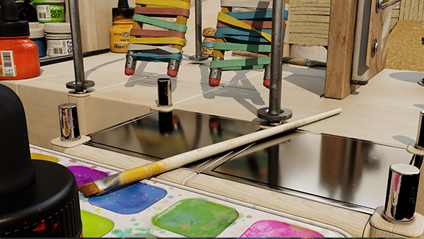
Available now, Kickstart RT makes it easier than ever to add real-time ray tracing to game engines, producing realistic reflections, shadows, ambient occlusion, and global illumination.
Figure 3. This scene highlights ray tracing, global illumination, ambient occlusion, and ray traced shadows, enabled through KickStart SDK.
Traditionally, game engines must bind all active materials in a scene. Kickstart RT delivers beautiful ray-traced effects, while foregoing legacy requirements and invasive changes to existing material systems.
Kickstart RT provides a convenient starting point for developers to quickly and easily include realistic dynamic lighting of complex scenes in their game engines in a much shorter timespan than traditional methods. It’s also helpful for those who may find upgrading their engine to the DirectX12 API difficult.
Make game testing faster and easier with GeForce NOW
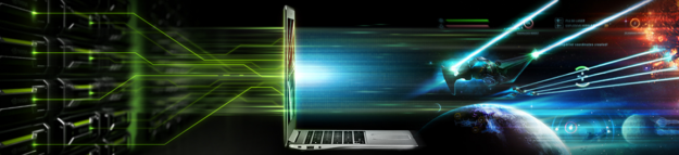
Figure 4. The NVIDIA GeForce NOW platform.
With a network of more than 30 data centers and 80 countries, GeForce NOW (GFN) uses the power of the cloud to take the GeForce PC gaming experience to any device. This extended infrastructure provides a developer platform for studios and publishers to perform their game development virtually, starting with playtesting.
With GeForce NOW Cloud Playtest, players and observers can be anywhere in the world. Game developers can upload a build to the cloud, and schedule a playtest for players and observers to manage on their calendar.
During a playtest session, a player uses the GFN app to play the targeted game, while streaming their camera and microphone. Observers watch the gameplay and webcam feeds from the cloud. Developers need innovative ways to perform this vital part of game development safely and securely. All this is possible with Cloud Playtest on the GeForce NOW Developer Platform.
Virtual world simulation technology is opening new portals for game developers. The NVIDIA Omniverse platform is bringing a new era of opportunities to game developers.
Users can plug into any layer of the modular Omniverse stack to build advanced tools that simplify workflows, integrate advanced AI and simulation technologies, or help connect complex production pipelines.
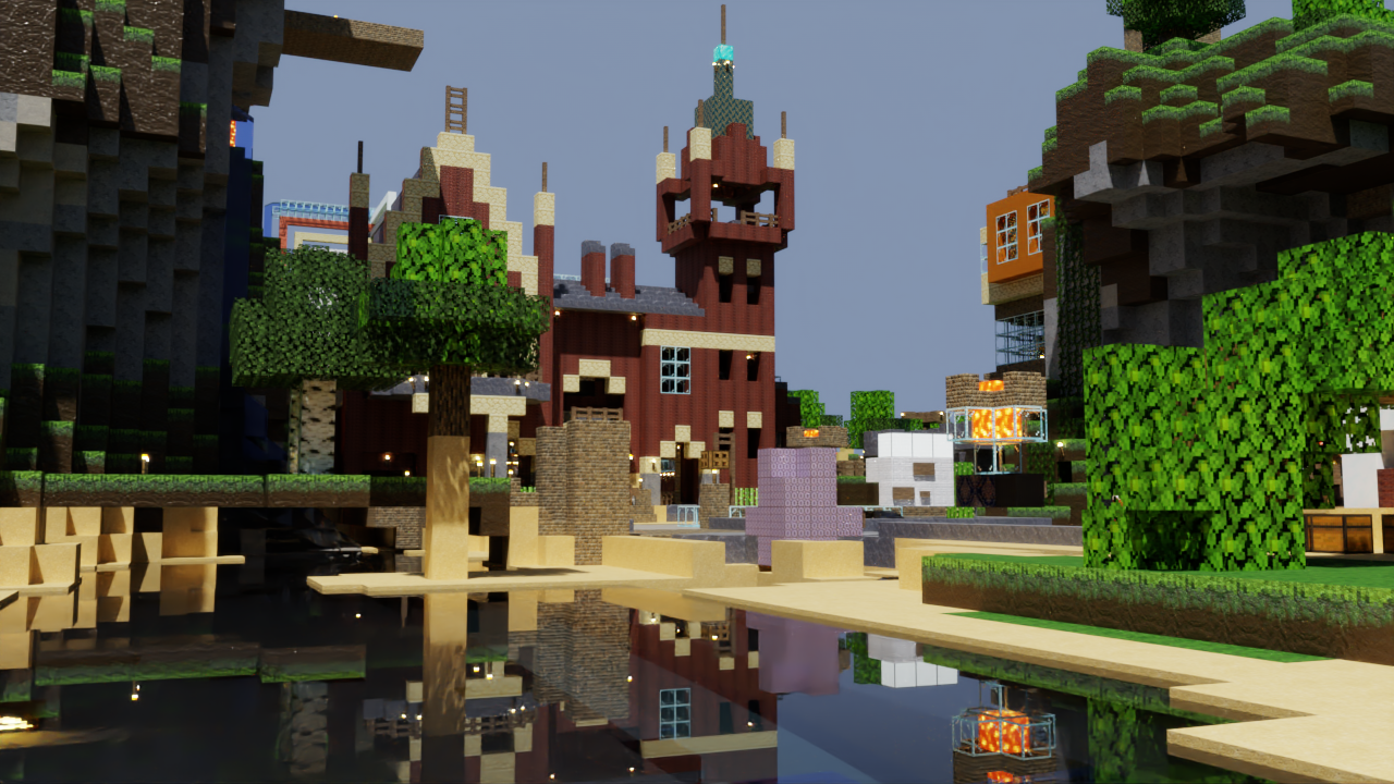
Figure 5. Game developers have been building virtual worlds for more than a decade (Minecraft pictured), courtesy of The Vokselians.
This GDC, see how Omniverse is supercharging game development pipelines with over 20 years of NVIDIA rendering, simulation, and AI technology.
Lastly, NVIDIA announced the #MadeInMachinima contest—where participants can remix iconic game characters into a cinematic short using the Omniverse Machinima app for a chance to win RTX-accelerated NVIDIA Studio laptops. Users can experiment with AI-enabled tools and create intuitively in real-time using assets from Squad, Mount & Blade II: Bannerlord, and Mechwarrior 5. The contest is free to enter.
It has never been easier to integrate real-time ray tracing in your games with Kickstart RT. However, for those looking for specific solutions, we’ve also updated our individual ray tracing SDKs.
The RTX Global Illumination plug-in is now available for Unreal Engine 5 (UE5). Developers can get a headstart in UE5 with dynamic lighting in their open worlds. Unreal Engine 4.27 has also been updated with performance and quality improvements while the plug-in for the NVIDIA branch of UE4 has received ray traced reflections and translucency support alongside skylight enhancements.
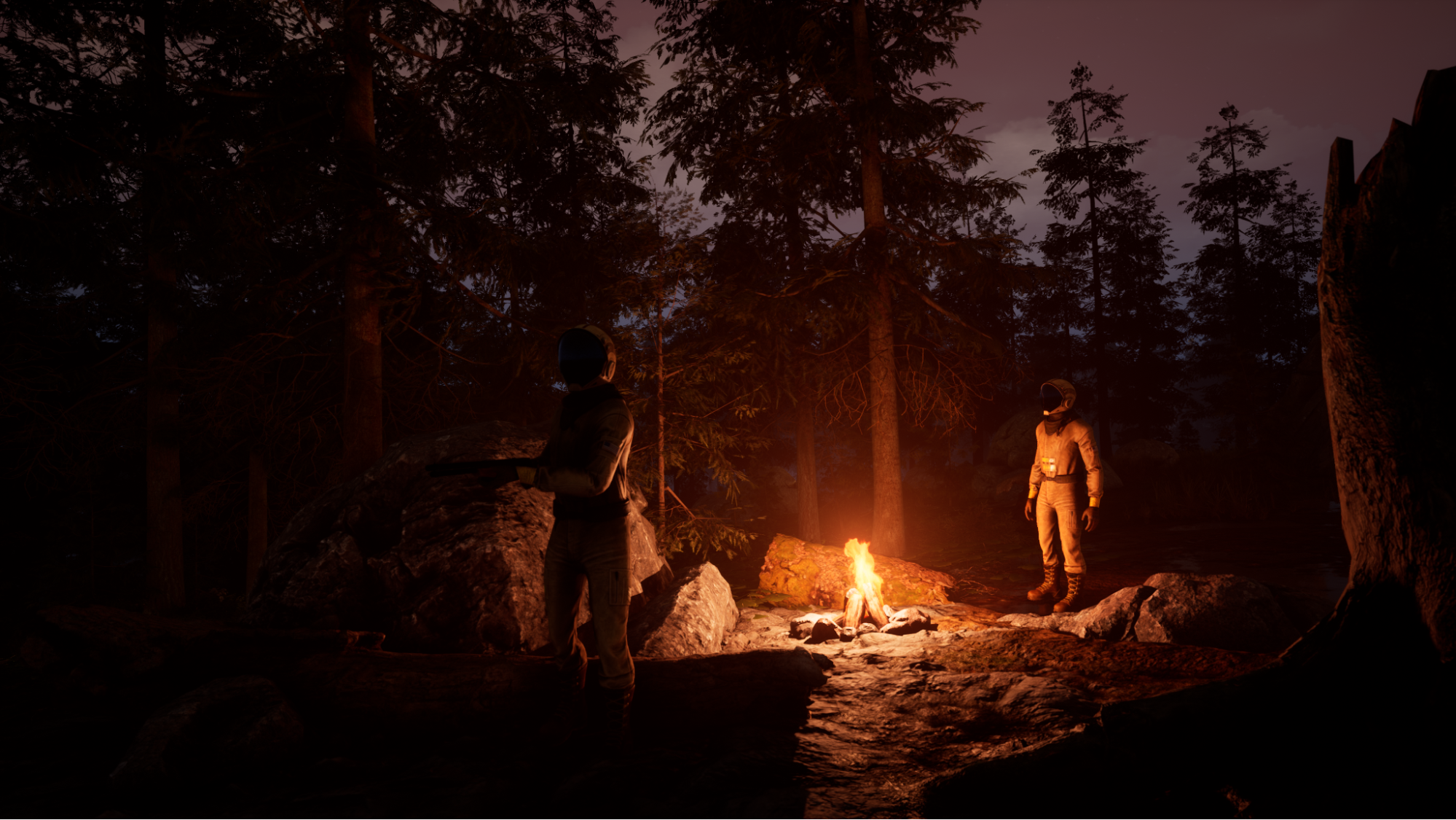
Figure 6. RTX highlighted in Icarus.
RTX Direct Illumination has received image quality improvements for glossy surfaces. NVIDIA Real-Time Denoisers introduces NVIDIA Image Scaling and a path-tracing mode within the sample application. It also has a new performance mode that is optimized for lower spec systems.
We’ve recently announced new latency measurement enhancements for NVIDIA Reflex that can be seen in Valorant, Overwatch, and Fortnite. These new features include per-frame PC Latency measurement and automatic configuration for Reflex Analyzer. Today, Reflex 1.6 SDK is available to all developers—making latency monitoring as easy as measuring FPS.
We’ve also updated our NVIDIA RTX Technology Showcase, an interactive demo, with Deep Learning Super Sampling (DLSS), Deep Learning Anti-Aliasing, and NVIDIA Image Scaling. Toggle different technologies to see the benefits AI can bring to your projects. For developers who have benefited from DLSS, we’ve updated the SDK to include a new and simpler way to integrate the latest NVIDIA technologies into your pipeline.
Latest tools and SDKs for XR development
Truly immersive XR games require advanced graphics, best-in-class lighting, and performance optimizations to run smoothly on all-in-one VR headsets. Cutting-edge XR solutions like NVIDIA CloudXR streaming and NVIDIA VRWorks are making it easier and faster for game developers to create amazing AR and VR experiences.
Developers and early access users can accurately capture and replay VR sessions for performance testing, scene troubleshooting, and more with NVIDIA Virtual Reality Capture and Replay (VCR).
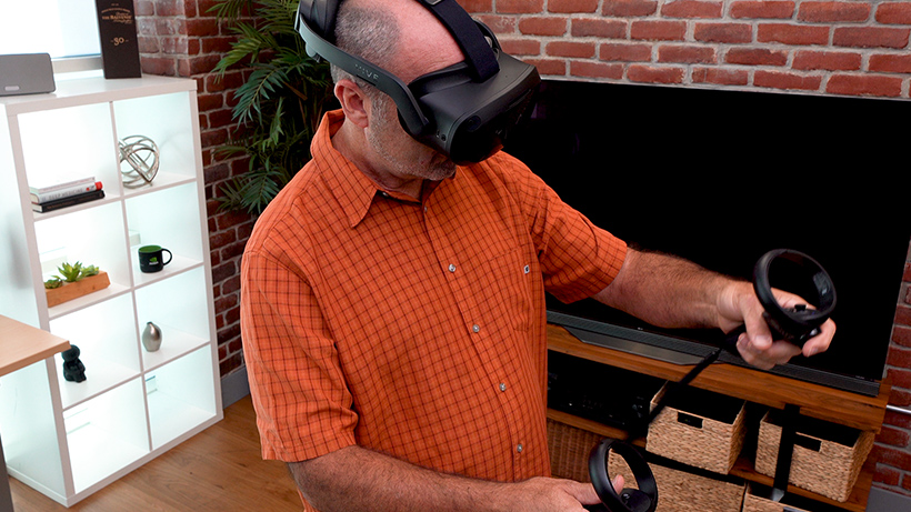
Figure 7. NVIDIA CloudXR streaming on an HTC VIVE
Attempting to repeat a user’s VR experience exactly is time consuming, and nearly impossible. VCR makes replaying VR sessions both accurate and painless. The tool records time-stamped HMD and controller inputs during an immersive VR session. Users can then replay the recording, without an HMD attached, to reproduce the session. It’s also possible to filter the recorded session through an optional processing step, cleaning up the data and removing excessive camera motion.
The latest Nsight Graphics 2022.2 features the brand new Ray Tracing Acceleration Structure Instance Heatmap and Shader Timing Heatmap. The GPU Trace Profiler has been improved to help developers see when GPU activity belonging to other processes may be interfering with profiling data. This ensures that the information that developers get for profiling is accurate and reliable
Figure 8. The latest version of Nsight Graphics is now available and includes numerous bug fixes, improvements and useful new features.
NVIDIA Nsight Systems is a triage and performance analysis tool designed to track GPU workloads to their CPU origins within a system-wide view. The new Nsight Systems 2022.2 release now includes support for Vulkan graphics pipeline library and Vulkan memory operations and warnings. Enhancements to multi report view further improve the ability to compare and debug issues.
Figure 9. Building the next great game with NVIDIA Nsight tools.
Game developers can find additional free resources to recreate fully ray-traced and AI-driven virtual worlds on the NVIDIA Game Development resources page. Check out NVIDIA GTC 2022 game development sessions from this past week.
A unifying goal of work like this is to develop new disease detection or monitoring approaches that are less invasive, more accurate, cheaper and more readily available. However, one restriction to potential broad population-level applicability of efforts to extract biomarkers from fundus photos is getting the fundus photos themselves, which requires specialized imaging equipment and a trained technician.
The eye can be imaged in multiple ways. A common approach for diabetic retinal disease screening is to examine the posterior segment using fundus photographs (left), which have been shown to contain signals of kidney and heart disease, as well as anemia. Another way is to take photographs of the front of the eye (external eye photos; right), which is typically used to track conditions affecting the eyelids, conjunctiva, cornea, and lens.
In “Detection of signs of disease in external photographs of the eyes via deep learning”, in press at Nature Biomedical Engineering, we show that a deep learning model can extract potentially useful biomarkers from external eye photos (i.e., photos of the front of the eye). In particular, for diabetic patients, the model can predict the presence of diabetic retinal disease, elevated HbA1c (a biomarker of diabetic blood sugar control and outcomes), and elevated blood lipids (a biomarker of cardiovascular risk). External eye photos as an imaging modality are particularly interesting because their use may reduce the need for specialized equipment, opening the door to various avenues of improving the accessibility of health screening.
Developing the Model To develop the model, we used de-identified data from over 145,000 patients from a teleretinal diabetic retinopathy screening program. We trained a convolutional neural network both on these images and on the corresponding ground truth for the variables we wanted the model to predict (i.e., whether the patient has diabetic retinal disease, elevated HbA1c, or elevated lipids) so that the neural network could learn from these examples. After training, the model is able to take external eye photos as input and then output predictions for whether the patient has diabetic retinal disease, or elevated sugars or lipids.
A schematic showing the model generating predictions for an external eye photo.
We measured model performance using the area under the receiver operator characteristic curve (AUC), which quantifies how frequently the model assigns higher scores to patients who are truly positive than patients who are truly negative (i.e., a perfect model scores 100%, compared to 50% for random guesses). The model detected various forms of diabetic retinal disease with AUCs of 71-82%, AUCs of 67-70% for elevated HbA1c, and AUCs of 57-68% for elevated lipids. These results indicate that, though imperfect, external eye photos can help detect and quantify various parameters of systemic health.
Much like the CDC’s pre-diabetes screening questionnaire, external eye photos may be able to help “pre-screen” people and identify those who may benefit from further confirmatory testing. If we sort all patients in our study based on their predicted risk and look at the top 5% of that list, 69% of those patients had HbA1c measurements ≥ 9 (indicating poor blood sugar control for patients with diabetes). For comparison, among patients who are at highest risk according to a risk score based on demographics and years with diabetes, only 55% had HbA1c ≥ 9, and among patients selected at random only 33% had HbA1c ≥ 9.
Assessing Potential Bias We emphasize that this is promising, yet early, proof-of-concept research showcasing a novel discovery. That said, because we believe that it is important to evaluate potential biases in the data and model, we undertook a multi-pronged approach for bias assessment.
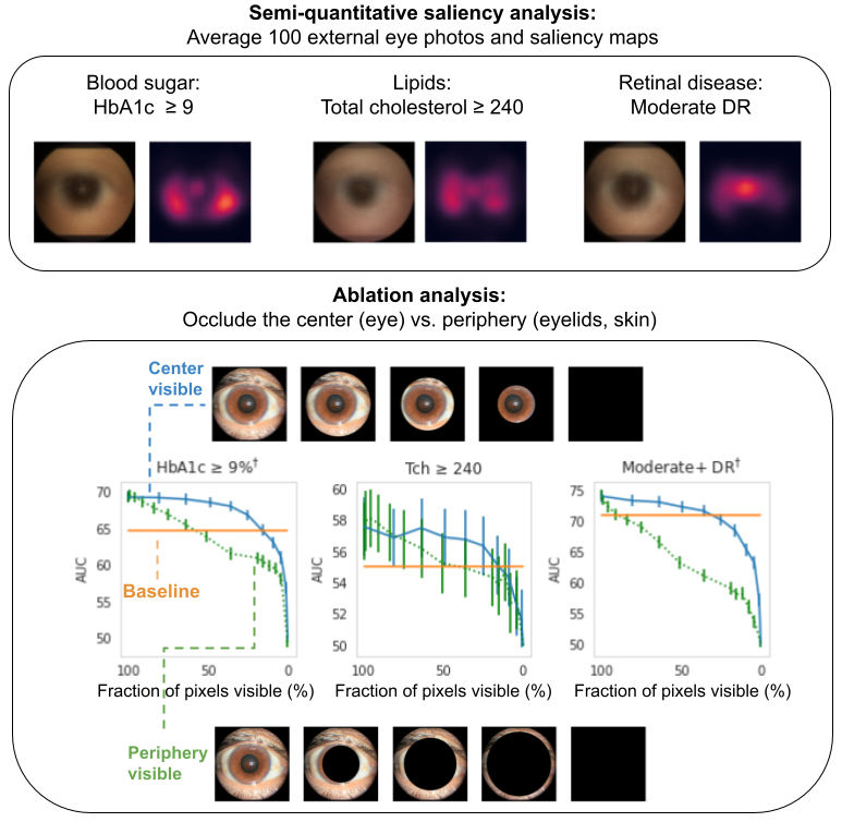
First, we conducted various explainability analyses aimed at discovering what parts of the image contribute most to the algorithm’s predictions (similar to our anemia work). Both saliency analyses (which examine which pixels most influenced the predictions) and ablation experiments (which examine the impact of removing various image regions) indicate that the algorithm is most influenced by the center of the image (the areas of the sclera, iris, and pupil of the eye, but not the eyelids). This is demonstrated below where one can see that the AUC declines much more quickly when image occlusion starts in the center (green lines) than when it starts in the periphery (blue lines).
Explainability analysis shows that (top) all predictions focused on different parts of the eye, and that (bottom) occluding the center of the image (corresponding to parts of the eyeball) has a much greater effect than occluding the periphery (corresponding to the surrounding structures, such as eyelids), as shown by the green line’s steeper decline. The “baseline” is a logistic regression model that takes self-reported age, sex, race and years with diabetes as input.
Second, our development dataset spanned a diverse set of locations within the U.S., encompassing over 300,000 de-identified photos taken at 301 diabetic retinopathy screening sites. Our evaluation datasets comprised over 95,000 images from 198 sites in 18 US states, including datasets of predominantly Hispanic or Latino patients, a dataset of majority Black patients, and a dataset that included patients without diabetes. We conducted extensive subgroup analyses across groups of patients with different demographic and physical characteristics (such as age, sex, race and ethnicity, presence of cataract, pupil size, and even camera type), and controlled for these variables as covariates. The algorithm was more predictive than the baseline in all subgroups after accounting for these factors.
Conclusion This exciting work demonstrates the feasibility of extracting useful health related signals from external eye photographs, and has potential implications for the large and rapidly growing population of patients with diabetes or other chronic diseases. There is a long way to go to achieve broad applicability, for example understanding what level of image quality is needed, generalizing to patients with and without known chronic diseases, and understanding generalization to images taken with different cameras and under a wider variety of conditions, like lighting and environment. In continued partnership with academic and nonacademic experts, including EyePACS and CGMH, we look forward to further developing and testing our algorithm on larger and more comprehensive datasets, and broadening the set of biomarkers recognized (e.g., for liver disease). Ultimately we are working towards making non-invasive health and wellness tools more accessible to everyone.
Acknowledgements This work involved the efforts of a multidisciplinary team of software engineers, researchers, clinicians and cross functional contributors. Key contributors to this project include: Boris Babenko, Akinori Mitani, Ilana Traynis, Naho Kitade, Preeti Singh, April Y. Maa, Jorge Cuadros, Greg S. Corrado, Lily Peng, Dale R. Webster, Avinash Varadarajan, Naama Hammel, and Yun Liu. The authors would also like to acknowledge Huy Doan, Quang Duong, Roy Lee, and the Google Health team for software infrastructure support and data collection. We also thank Tiffany Guo, Mike McConnell, Michael Howell, and Sam Kavusi for their feedback on the manuscript. Last but not least, gratitude goes to the graders who labeled data for the pupil segmentation model, and a special thanks to Tom Small for the ideation and design that inspired the animation used in this blog post.
1The information presented here is research and does not reflect a product that is available for sale. Future availability cannot be guaranteed. ↩
Developers and users can capture and replay VR sessions for performance testing and scene troubleshooting with early access to NVIDIA Virtual Reality Capture and Replay.
Developers and early access users can now accurately capture and replay VR sessions for performance testing, scene troubleshooting, and more with NVIDIA Virtual Reality Capture and Replay (VCR.)
The potentials of virtual worlds are limitless, but working with VR content poses challenges, especially when it comes to recording or recreating a virtual experience. Unlike the real world, capturing an immersive scene isn’t as easy as taking a video on your phone or hitting the record button on your computer.
It’s impossible to repeat an identical experience in VR, and immersive demos are often jittery and difficult to watch due to excessive camera motion. Creating VR applications can also be cumbersome, as developers have to jump in and out of their headsets to code, test, and refine their work. Plus, all of these tasks require a 1:1 device connection, in order to launch and run a VR application.
All of this makes recording anything in VR an extremely time-consuming and tedious process.
“We often find ourselves spending more time getting the hardware ready and navigating to a location within VR than we actually do testing or troubleshooting an issue,” explains Lukas Faeth, Senior Product Manager at Autodesk. “The NVIDIA VCR SDK should help us test performance between builds without having to put someone in VR for hours at a time.”
“The NVIDIA VCR SDK seems at first promising and rather cool, and when I tried it out it left my head spinning! With a little creative thought, this tool can be very powerful. I am still trying to get my head around the myriad of ways I can use it in my day-to-day workflows. It has opened up quite a few use cases for me in terms of automatic testing, training potential VR users, and creating high-quality GI renders of an OpenGL VR session,” said Danny Tierney, Automotive Design Solution Specialist at Autodesk
Easier, faster VR video production
NVIDIA VCR started as an internal project for VR performance testing across NVIDIA GPUs. The NVIDIA XR team continued to expand the feature set as they recognized new use cases. The team is making it available to select partners to help evaluate, test, and identify additional applications for the project.
Figure 1. Potential NVIDIA VCR use cases: Performance testing, scene troubleshooting, and VR video generation.
With NVIDIA VCR, developers and creators can more easily develop VR applications, assist end users with QA and troubleshooting, and generate quality VR videos.
NVIDIA VCR features include:
Accurate and painless VR session playback. This is especially useful for performance testing and QC.
Less time in a headset. With a reduced number of development steps users spend less time jumping in and out of VR.
Multirole recordings from a single headset in the same VR scene using one HMD. Replay the recordings simultaneously to simulate collaboration.
Early partners like ESI Group imagine promising opportunities to leverage the SDK. “NVIDIA VCR opens up infinite possibilities for immersive experiences,” says Eric Kam, Solutions Marketing Manager at ESI Group.
“Recording and playback of virtuality add a temporal dimension to VR sessions,” Kam adds, pointing out that VCR could be developed to serve downstream workflows in addition to addressing challenges with performance testing.
Getting started with NVIDIA VCR
NVIDIA VCR records time-stamped HMD and controller inputs during an immersive VR session. Users can then replay the recording, without an HMD attached, to reproduce the session. It’s also possible to filter the recorded session through an optional processing step, cleaning up the data and removing excessive camera motion.
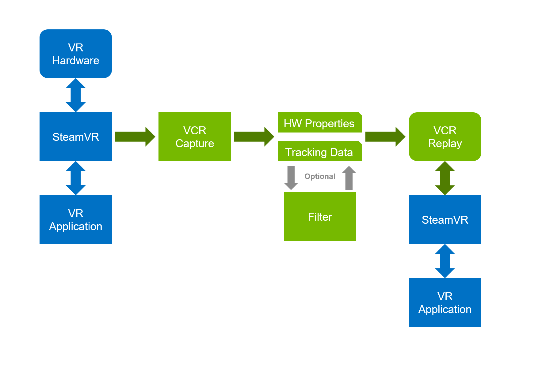
Figure 2. NVIDIA VCR workflow to capture, filter, and replay VR content.
Components of NVIDIA VCR:
Capture is an OpenVR background application that stores HMD and controller properties and logs motion and button presses into tracking data.
Filter is an optional processing step to read and write recorded sessions. Using the VCR C++ API, developers can analyze a session, clean up data, or retime HMD motion paths.
Replay uses an OpenVR driver to emulate an HMD and controllers, read tracking data, and replay motion and button presses in the scene. Hardware properties such as display resolution and refresh rate can be edited as a JSON file.
Four NVIDIA VCR Use Cases
Use a simple capture and replay workflow to record tracking data and replay it an infinite number of times. This is ideal for verifying scene correctness, such as in performance testing or QC use cases.
Video 1. Example of a simple capture and replay scenario.
In a filtering workflow, apply motion data smoothing to minimize jitter and produce a more professional-looking VR demo video or tutorial.
Video 2. Filtering a VCR session to reduce jitter.
Repeat and mix segments captured in VCR to generate an entirely new sequence. In the video below, the same set of segments (the letters “H,” “o,” “l,” and “e” in addition to movement and interaction data) were reordered to spell a completely new word.
Video 3. How to repeat and mix segments captured in VCR.
Use NVIDIA VCR within the Autodesk VRED application to capture an example of single-user collaboration. In this workflow, one user generates four separate VCR captures with a single HMD system. These were then replayed simultaneously on multiple systems to simulate multiuser collaboration.
Video 4. Building a collaborative scene in VCR using a single HMD system.
Apply to become an early access partner
NVIDIA VCR is available to a limited number of early access partners. If you have an innovative use case and are willing to provide feedback on VCR apply for early access.
This GTC focused roundup features updates to the HPC SDK, cuQuantum SDK, Nsight Graphics and Systems 2022.2, CUDA 11.6, Update 1, cuNumeric, and Warp.
Our weekly roundup covers the most recent software updates, learning resources, events, and notable news. This week we have several software releases.
Software releases
Leveraging standard languages for portable and performant code with the HPC SDK
The NVIDIA HPC SDK is a comprehensive suite of compilers, libraries, and tools for developing accelerated HPC applications. With a breadth of flexible support options, users can create applications with a programming model most relevant to their situation.
The HPC SDK offers a variety of programming models including performance-optimized drop-in libraries, standard languages, directives-based methods, and specialization provided by CUDA. Many of the latest enhancements have been in the area of standard language support for ISO C++, ISO Fortran, and Python.
The NVIDIA HPC compilers use recent advances in the public specifications for these languages, delivering a productive programming environment that is both portable and performant for scaling on GPU accelerated platforms.
Visit our site to download the new HPC SDK version 22.3 and read our new post on parallel programming with standard languages under our “Resources” section.
Accelerate quantum circuit simulation with the NVIDIA cuQuantum SDK
cuQuantum – An SDK for accelerating quantum circuit simulation NVIDIA cuQuantum is an SDK of optimized libraries and tools for accelerating quantum computing workflows. Developers can use cuQuantum while creating and verifying new algorithms more easily and reliably. Speeding up quantum circuit simulations by orders of magnitude, for both state vector and tensor network methods helps developers simulate bigger problems, faster.
Expanding ecosystem integrations and collaborations cuQuantum is now integrated as a backend in popular industry simulators. It is also offered as a part of quantum application development platforms, and is used to power quantum research at scale in areas from chemistry to climate modeling.
SDK available with new appliance beta The cuQuantum SDK is now GA and free to download. NVIDIA has also packaged up an optimized Beta software container, the cuQuantum DGX appliance, available from the NGC Catalog.
Boost ray tracing application performance using Nsight Graphics 2022.2
Nsight Graphics is a performance analysis tool designed to visualize, analyze, and optimize programming models. It also tunes to scale efficiently across any quantity or size of CPUs and GPUs—from workstations to supercomputers.
The latest features in Nsight Graphics 2022.2 include:
Simplify system profiling and debugging with Nsight Systems 2022.2
Nsight Systems is a triage and performance analysis tool designed to track GPU workloads to their CPU origins within a system-wide view. The features help you analyze your applications’ GPU utilization, graphic and compute API activity, and OS runtime operations. This helps optimize your application to perform and scale efficiently across any quantity or size of CPUs and GPUs—from workstations to supercomputers.
Enhanced CUDA 11.6, Update 1, platform for all new SDKs
This CUDA Toolkit release focuses on enhancing the programming model and performance of CUDA applications. CUDA 11.6 ships with the R510 driver, an update branch. CUDA Toolkit 11.6, Update 1, is available to download.
What’s new:
GSP driver architecture is now default on NVIDIA Turing and Ampere GPUs.
New API for disabling nodes in instantiated graph.
Deliver distributed and accelerated computing to Python with the help of cuNumeric
NVIDIA cuNumeric is a Legate library that aspires to provide a drop-in replacement for the NumPy API on top of the Legion runtime. This brings distributed and accelerated computing on the NVIDIA platform to the Python community.
What’s new:
Transparently accelerates and scales existing NumPy workflow
Scales to up to thousands of GPUs optimally
Requires zero code changes to ensure developer productivity
Warp helps Python coders with GPU-accelerated graphics simulation
Warp is a Python framework that gives coders an easy way to write GPU-accelerated, kernel-based programs in NVIDIA Omniverse and OmniGraph. With Warp, Omniverse developers can create GPU-accelerated, 3D simulation workflows and fantastic virtual worlds!
What’s new:
Kernel-based code in Python
Differentiable programming
Built-in geometry processing
Simulation performance on par with native code
Shorter time to market with improved iteration time
Discobox is a weakly supervised learning algorithm to identify objects without costly mask annotations during training.
Instance segmentation is a core visual recognition problem for detecting and segmenting objects. In the past several years, this area has been one of the holy grails in the computer vision community with wide applications ranging from autonomous vehicles (AV), robotics, video analysis, smart home, digital human, and healthcare.
Annotation, the process of classifying every object in an image or video, is a challenging component of instance segmentation. Training a conventional instance segmentation method, such as Mask R-CNN, requires class labels, bounding boxes, and segmentation masks of objects simultaneously.
However, obtaining segmentation masks is costly and time-consuming. The COCO dataset for example required about 70,000 hours of time to annotate 200k images, with 55,000 hours spent gathering object masks.
Introducing Discobox
Working to expedite the annotation process, NVIDIA researchers developed the DiscoBox framework. The solution uses a weakly supervised learning algorithm that can output high-quality instance segmentation without mask annotations during training.
The framework generates instance segmentation directly from bounding box supervisions, rather than using mask annotations to directly supervise the task. Bounding boxes were introduced as a fundamental form of annotation for training modern object detectors and use labeled rectangles to tightly enclose objects. Each rectangle encodes the localization, size, and category information of an object.
Bounding box annotation is the sweet spot of industrial computer vision applications. It contains rich localization information and is very easy to draw, making it more affordable and scalable when annotating large amounts of data. However, by itself, it does not provide pixel-level information, and cannot be directly used for training instance segmentation.
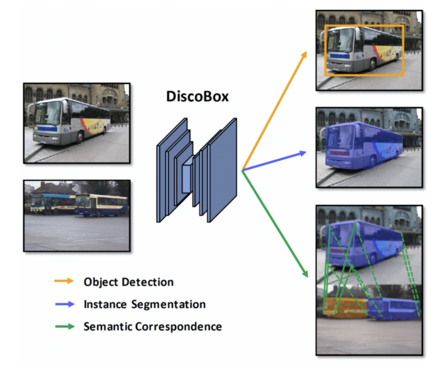
Figure 1. Given a pair of input images, DiscoBox is able to jointly output detection, instance segmentation, and multi-object semantic correspondence.
Innovative features of DiscoBox
DiscoBox is the first weakly supervised instance segmentation algorithm that gives comparable performance to fully-supervised methods while reducing labeling time and costs. The method, for example, is faster and more accurate than the legendary Mask R-CNN, without requiring mask annotations during training. This raises the question of whether mask annotations are truly needed in future instance segmentation applications as less labeling is required.
DiscoBox is also the first weakly supervised algorithm that unifies both instance segmentation and multi-object semantic correspondence under box supervision. These two tasks are useful in many computer vision applications such as 3D reconstruction and are shown to mutually help each other. For example, predicted object masks from instance segmentation can help semantic correspondence to focus on foreground object pixels, whereas semantic correspondence can refine mask prediction. DiscoBox unifies both tasks under box supervision, making their model training easy and scalable.
At the center of DiscoBox is a teacher-student design. The design features the use of self-consistency as a self-supervision to replace the mask supervision missing in DiscoBox training. The design is effective in promoting high-quality mask prediction, even though mask annotations are absent in training.
DiscoBox applications
There are many applications of DiscoBox beyond its use as an auto-labeling toolkit for AI applications at NVIDIA. By automating costly mask annotations the tool could help product teams in intelligent video analytics or AV save a significant amount on annotation budgets.
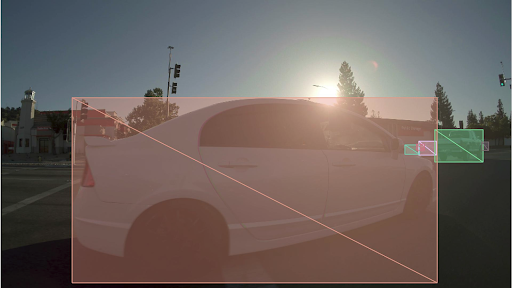
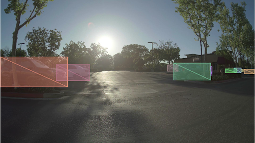
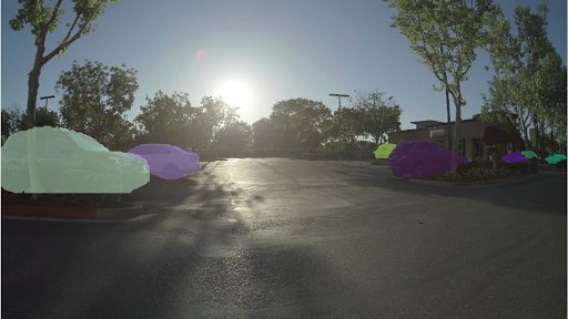
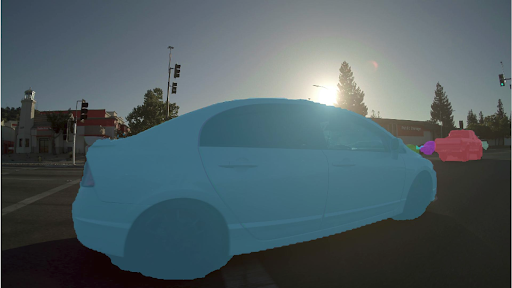
Figure 2. DiscoBox auto-labeling cars in an autonomous vehicle computer vision test.
Another potential application is 3D reconstruction, an area where both object masks and semantic correspondence are important information for a reconstruction task. DiscoBox is capable of giving these two outputs with only bounding box supervision, helping generate large-scale 3D reconstruction in an open-world scenario. This could benefit many applications for building virtual worlds, such as content creation, virtual reality, and digital humans.
For more information on the model or to use the code, visit DiscoBox on GitHub.
To learn more about research NVIDIA is conducting, visit NVIDIA Research.
The hum of a bustling data center is music to an AI developer’s ears — and NVIDIA data centers have found a rhythm of their own, grooving to the swing classic “Sing, Sing, Sing” in this week’s GTC keynote address. The lighthearted video, created with the NVIDIA Omniverse platform, features Louis Prima’s iconic music track, Read article >
GeForce NOW gives you the power to game almost anywhere, at GeForce quality. And with the latest controller from SteelSeries, members can stay in control of the action on Android and Chromebook devices. This GFN Thursday takes a look at the SteelSeries Stratus+, now part of the GeForce NOW Recommended program. And it wouldn’t be Read article >
From the documentation and forum discussions, I learnt that these embeddings are the output of a pretrained model (MFCC+CNN) of the 10 second chunks of respective youtube videos. I have also learnt that these embeddings make it easy to work on deep learning models. How does it help the ML engineers?
My confusion is if these audio embeddings are already pre-trained, what are the utilities of these audio embeddings? i.e. How can I use these embeddings to train advanced models for performing Sound Event Detection?

 NVIDIA announced a number of new tools for game developers at this year’s GDC to help you save time, more easily integrate RTX, and simplify the creation of virtual worlds.
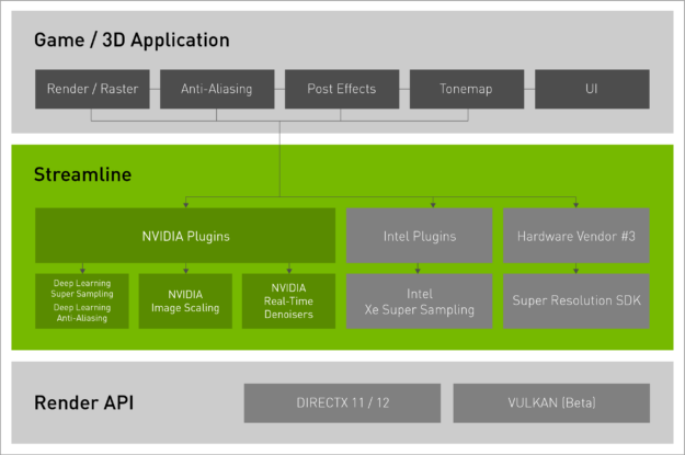


 Developers and users can capture and replay VR sessions for performance testing and scene troubleshooting with early access to NVIDIA Virtual Reality Capture and Replay.
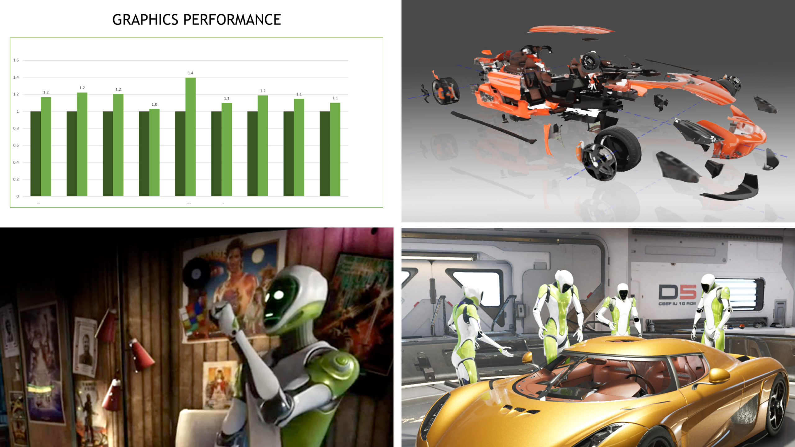
 This GTC focused roundup features updates to the HPC SDK, cuQuantum SDK, Nsight Graphics and Systems 2022.2, CUDA 11.6, Update 1, cuNumeric, and Warp.
 Discobox is a weakly supervised learning algorithm to identify objects without costly mask annotations during training.