
The Kroger Co. (NYSE: KR) and NVIDIA today announced a strategic collaboration to reimagine the shopping experience using AI-enabled applications and services.
Remote work and hybrid workplaces are the new normal for professionals in many industries. Teams spread throughout the world are expected to create and collaborate while maintaining top productivity and performance. Businesses use the NVIDIA RTX platform to enable their workers to keep up with the most demanding workloads, from anywhere. And today, NVIDIA is Read article >
The post New NVIDIA RTX GPUs Tackle Demanding Professional Workflows and Hybrid Work, Enabling Creation From Anywhere appeared first on NVIDIA Blog.
The University of Florida’s academic health center, UF Health, has teamed up with NVIDIA to develop a neural network that generates synthetic clinical data — a powerful resource that researchers can use to train other AI models in healthcare. Trained on a decade of data representing more than 2 million patients, SynGatorTron is a language Read article >
The post Unlimited Data, Unlimited Possibilities: UF Health and NVIDIA Build World’s Largest Clinical Language Generator appeared first on NVIDIA Blog.
Promising to transform trillion-dollar industries and address the “grand challenges” of our time, NVIDIA founder and CEO Jensen Huang Tuesday shared a vision of an era where intelligence is created on an industrial scale and woven into real and virtual worlds. Kicking off NVIDIA’s GTC conference, Huang introduced new silicon — including the new Hopper Read article >
The post Turning Data Centers into ‘AI Factories’: NVIDIA CEO Introduces Hopper Architecture, H100 GPU, New Supercomputers and Software appeared first on NVIDIA Blog.
Categories
NVIDIA Hopper Architecture In-Depth
 Everything you want to know about the new H100 GPU.
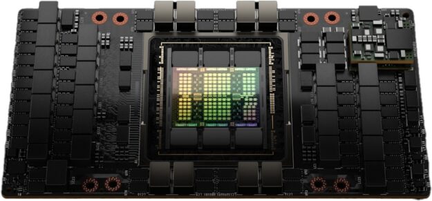
Today during the 2022 NVIDIA GTC Keynote address, NVIDIA CEO Jensen Huang introduced the new NVIDIA H100 Tensor Core GPU based on the new NVIDIA Hopper GPU architecture. This post gives you a look inside the new H100 GPU and describes important new features of NVIDIA Hopper architecture GPUs.
Introducing the NVIDIA H100 Tensor Core GPU
The NVIDIA H100 Tensor Core GPU is our ninth-generation data center GPU designed to deliver an order-of-magnitude performance leap for large-scale AI and HPC over the prior-generation NVIDIA A100 Tensor Core GPU. H100 carries over the major design focus of A100 to improve strong scaling for AI and HPC workloads, with substantial improvements in architectural efficiency.
For today’s mainstream AI and HPC models, H100 with InfiniBand interconnect delivers up to 30x the performance of A100. The new NVLink Switch System interconnect targets some of the largest and most challenging computing workloads that require model parallelism across multiple GPU-accelerated nodes to fit. These workloads receive yet another generational performance leap, in some cases tripling performance yet again over H100 with InfiniBand.
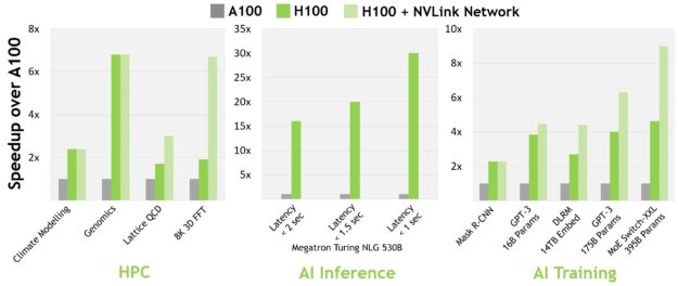
All performance numbers are preliminary, based on current expectations and subject to change in shipping products. A100 cluster: HDR IB network. H100 cluster: NDR IB network with NVLink Switch System where indicated. # GPUs: Climate Modeling 1K, LQCD 1K, Genomics 8, 3D-FFT 256, MT-NLG 32 (batch sizes: 4 for A100, 60 for H100 at 1 sec, 8 for A100 and 64 for H100 at 1.5 and 2sec), MRCNN 8 (batch 32),GPT-3 16B 512 (batch 256), DLRM 128 (batch 64K), GPT-3 16K (batch 512), MoE 8K (batch 512, one expert per GPU).
At GTC Spring 2022, the new NVIDIA Grace Hopper Superchip product was announced. The NVIDIA Hopper H100 Tensor Core GPU will power the NVIDIA Grace Hopper Superchip CPU+GPU architecture, purpose-built for terabyte-scale accelerated computing and providing 10x higher performance on large-model AI and HPC.
The NVIDIA Grace Hopper Superchip leverages the flexibility of the Arm architecture to create a CPU and server architecture designed from the ground up for accelerated computing. H100 is paired to the NVIDIA Grace CPU with the ultra-fast NVIDIA chip-to-chip interconnect, delivering 900 GB/s of total bandwidth, 7x faster than PCIe Gen5. This innovative design delivers up to 30x higher aggregate bandwidth compared to today’s fastest servers and up to 10x higher performance for applications using terabytes of data.
NVIDIA H100 GPU key feature summary
- The new streaming multiprocessor (SM) has many performance and efficiency improvements. Key new features include:
- New fourth-generation Tensor Cores are up to 6x faster chip-to-chip compared to A100, including per-SM speedup, additional SM count, and higher clocks of H100. On a per SM basis, the Tensor Cores deliver 2x the MMA (Matrix Multiply-Accumulate) computational rates of the A100 SM on equivalent data types, and 4x the rate of A100 using the new FP8 data type, compared to previous generation 16-bit floating-point options. The Sparsity feature exploits fine-grained structured sparsity in deep learning networks, doubling the performance of standard Tensor Core operations
- New DPX Instructions accelerate dynamic programming algorithms by up to 7x over the A100 GPU. Two examples include the Smith-Waterman algorithm for genomics processing, and the Floyd-Warshall algorithm used to find optimal routes for a fleet of robots through a dynamic warehouse environment.
- 3x faster IEEE FP64 and FP32 processing rates chip-to-chip compared to A100, due to 2x faster clock-for-clock performance per SM, plus additional SM counts and higher clocks of H100.
- New thread block cluster feature enables programmatic control of locality at a granularity larger than a single thread block on a single SM. This extends the CUDA programming model by adding another level to the programming hierarchy to now include threads, thread blocks, thread block clusters, and grids. Clusters enable multiple thread blocks running concurrently across multiple SMs to synchronize and collaboratively fetch and exchange data.
- Distributed shared memory allows direct SM-to-SM communications for loads, stores, and atomics across multiple SM shared memory blocks.
- New asynchronous execution features include a new Tensor Memory Accelerator (TMA) unit that can transfer large blocks of data efficiently between global memory and shared memory. TMA also supports asynchronous copies between thread blocks in a cluster. There is also a new asynchronous transaction barrier for doing atomic data movement and synchronization.
- New transformer engine uses a combination of software and custom NVIDIA Hopper Tensor Core technology designed specifically to accelerate transformer model training and inference. The transformer engine intelligently manages and dynamically chooses between FP8 and 16-bit calculations, automatically handling re-casting and scaling between FP8 and 16-bit in each layer to deliver up to 9x faster AI training and up to 30x faster AI inference speedups on large language models compared to the prior generation A100.
- HBM3 memory subsystem provides nearly a 2x bandwidth increase over the previous generation. The H100 SXM5 GPU is the world’s first GPU with HBM3 memory delivering a class-leading 3 TB/sec of memory bandwidth.
- 50 MB L2 cache architecture caches large portions of models and datasets for repeated access, reducing trips to HBM3.
- Second-generation Multi-Instance GPU (MIG) technology provides approximately 3x more compute capacity and nearly 2x more memory bandwidth per GPU instance compared to A100. Confidential Computing capability with MIG-level TEE is now provided for the first time. Up to seven individual GPU instances are supported, each with dedicated NVDEC and NVJPG units. Each instance now includes its own set of performance monitors that work with NVIDIA developer tools.
- New Confidential Computing support protects user data, defends against hardware and software attacks, and better isolates and protects virtual machines (VMs) from each other in virtualized and MIG environments. H100 implements the world’s first native Confidential Computing GPU and extends the trusted execution environment (TEE) with CPUs at full PCIe line rate.
- Fourth-generation NVIDIA NVLink provides a 3x bandwidth increase on all-reduce operations and a 50% general bandwidth increase over the prior generation NVLink with 900 GB/sec total bandwidth for multi-GPU IO operating at 7x the bandwidth of PCIe Gen 5.
- Third-generation NVSwitch technology includes switches residing both inside and outside of nodes to connect multiple GPUs in servers, clusters, and data center environments. Each NVSwitch inside a node provides 64 ports of fourth-generation NVLink links to accelerate multi-GPU connectivity. Total switch throughput increases to 13.6 Tbits/sec from 7.2 Tbits/sec in the prior generation. New third-generation NVSwitch technology also provides hardware acceleration for collective operations with multicast and NVIDIA SHARP in-network reductions.
- New NVLink Switch System interconnect technology and new second-level NVLink Switches based on third-gen NVSwitch technology introduce address space isolation and protection, enabling up to 32 nodes or 256 GPUs to be connected over NVLink in a 2:1 tapered, fat tree topology. These connected nodes are capable of delivering 57.6 TB/sec of all-to-all bandwidth and can supply an incredible one exaFLOP of FP8 sparse AI compute.
- PCIe Gen 5 provides 128 GB/sec total bandwidth (64 GB/sec in each direction) compared to 64 GB/sec total bandwidth (32GB/sec in each direction) in Gen 4 PCIe. PCIe Gen 5 enables H100 to interface with the highest performing x86 CPUs and SmartNICs or data processing units (DPUs).
Many other new features are also included to improve strong scaling, reduce latencies and overheads, and generally simplify GPU programming.
NVIDIA H100 GPU architecture in-depth
The NVIDIA H100 GPU based on the new NVIDIA Hopper GPU architecture features multiple innovations:
- New fourth-generation Tensor Cores perform faster matrix computations than ever before on an even broader array of AI and HPC tasks.
- A new transformer engine enables H100 to deliver up to 9x faster AI training and up to 30x faster AI. inference speedups on large language models compared to the prior generation A100.
- The new NVLink Network interconnect enables GPU-to-GPU communication among up to 256 GPUs across multiple compute nodes.
- Secure MIG partitions the GPU into isolated, right-size instances to maximize quality of service (QoS) for smaller workloads.
Numerous other new architectural features enable many applications to attain up to 3x performance improvement.
NVIDIA H100 is the first truly asynchronous GPU. H100 extends A100’s global-to-shared asynchronous transfers across all address spaces and adds support for tensor memory access patterns. It enables applications to build end-to-end asynchronous pipelines that move data into and off the chip, completely overlapping and hiding data movement with computation.
Only a small number of CUDA threads are now required to manage the full memory bandwidth of H100 using the new Tensor Memory Accelerator, while most other CUDA threads can be focused on general-purpose computations, such as pre-processing and post-processing data for the new generation of Tensor Cores.
H100 grows the CUDA thread group hierarchy with a new level called the thread block cluster. A cluster is a group of thread blocks that are guaranteed to be concurrently scheduled, and enable efficient cooperation and data sharing for threads across multiple SMs. A cluster also cooperatively drives asynchronous units like the Tensor Memory Accelerator and the Tensor Cores more efficiently.
Orchestrating the growing number of on-chip accelerators and diverse groups of general-purpose threads requires synchronization. For example, threads and accelerators that consume outputs must wait on threads and accelerators that produce them.
NVIDIA asynchronous transaction barriers enables general-purpose CUDA threads and on-chip accelerators within a cluster to synchronize efficiently, even if they reside on separate SMs. All these new features enable every user and application to use all units of their H100 GPUs fully at all times, making H100 the most powerful, most programmable, and power-efficient NVIDIA GPU to date.
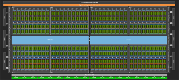
The full GH100 GPU that powers the H100 GPU is fabricated using the TSMC 4N process customized for NVIDIA, with 80 billion transistors, a die size of 814 mm2, and higher frequency design.
The NVIDIA GH100 GPU is composed of multiple GPU processing clusters (GPCs), texture processing clusters (TPCs), streaming multiprocessors (SMs), L2 cache, and HBM3 memory controllers.
The full implementation of the GH100 GPU includes the following units:
- 8 GPCs, 72 TPCs (9 TPCs/GPC), 2 SMs/TPC, 144 SMs per full GPU
- 128 FP32 CUDA Cores per SM, 18432 FP32 CUDA Cores per full GPU
- 4 fourth-generation Tensor Cores per SM, 576 per full GPU
- 6 HBM3 or HBM2e stacks, 12 512-bit memory controllers
- 60 MB L2 cache
- Fourth-generation NVLink and PCIe Gen 5
The NVIDIA H100 GPU with SXM5 board form-factor includes the following units:
- 8 GPCs, 66 TPCs, 2 SMs/TPC, 132 SMs per GPU
- 128 FP32 CUDA Cores per SM, 16896 FP32 CUDA Cores per GPU
- 4 fourth-generation Tensor Cores per SM, 528 per GPU
- 80 GB HBM3, 5 HBM3 stacks, 10 512-bit memory controllers
- 50 MB L2 cache
- Fourth-generation NVLink and PCIe Gen 5
The NVIDIA H100 GPU with a PCIe Gen 5 board form-factor includes the following units:
- 7 or 8 GPCs, 57 TPCs, 2 SMs/TPC, 114 SMs per GPU
- 128 FP32 CUDA Cores/SM, 14592 FP32 CUDA Cores per GPU
- 4 fourth-generation Tensor Cores per SM, 456 per GPU
- 80 GB HBM2e, 5 HBM2e stacks, 10 512-bit memory controllers
- 50 MB L2 cache
- Fourth-generation NVLink and PCIe Gen 5
Using the TSMC 4N fabrication process enables H100 to increase GPU core frequency, improve performance per watt, and incorporate more GPCs, TPCs, and SMs than the prior generation GA100 GPU, which was based on the TSMC 7nm N7 process.
Figure 3 shows a full GH100 GPU with 144 SMs. The H100 SXM5 GPU has 132 SMs, and the PCIe version has 114 SMs. The H100 GPUs are primarily built for executing data center and edge compute workloads for AI, HPC, and data analytics, but not graphics processing. Only two TPCs in both the SXM5 and PCIe H100 GPUs are graphics-capable (that is, they can run vertex, geometry, and pixel shaders).
H100 SM architecture
Building upon the NVIDIA A100 Tensor Core GPU SM architecture, the H100 SM quadruples the A100 peak per SM floating point computational power due to the introduction of FP8, and doubles the A100 raw SM computational power on all previous Tensor Core, FP32, and FP64 data types, clock-for-clock.
The new Transformer Engine, combined with NVIDIA Hopper FP8 Tensor Cores, delivers up to 9x faster AI training and 30x faster AI inference speedups on large language models compared to the prior generation A100. The new NVIDIA Hopper DPX instructions enable up to 7x faster Smith-Waterman algorithm processing for genomics and protein sequencing.
The new NVIDIA Hopper fourth-generation Tensor Core, Tensor Memory Accelerator, and many other new SM and general H100 architecture improvements together deliver up to 3x faster HPC and AI performance in many other cases.
| NVIDIA H100 SXM51 | NVIDIA H100 PCIe1 | |
| Peak FP641 | 30 TFLOPS | 24 TFLOPS |
| Peak FP64 Tensor Core1 | 60 TFLOPS | 48 TFLOPS |
| Peak FP321 | 60 TFLOPS | 48 TFLOPS |
| Peak FP161 | 120 TFLOPS | 96 TFLOPS |
| Peak BF161 | 120 TFLOPS | 96 TFLOPS |
| Peak TF32 Tensor Core1 | 500 TFLOPS | 1000 TFLOPS2 | 400 TFLOPS | 800 TFLOPS2 |
| Peak FP16 Tensor Core1 | 1000 TFLOPS | 2000 TFLOPS2 | 800 TFLOPS | 1600 TFLOPS2 |
| Peak BF16 Tensor Core1 | 1000 TFLOPS | 2000 TFLOPS2 | 800 TFLOPS | 1600 TFLOPS2 |
| Peak FP8 Tensor Core1 | 2000 TFLOPS | 4000 TFLOPS2 | 1600 TFLOPS | 3200 TFLOPS2 |
| Peak INT8 Tensor Core1 | 2000 TOPS | 4000 TOPS2 | 1600 TOPS | 3200 TOPS2 |
- Preliminary performance estimates for H100 based on current expectations and subject to change in the shipping products
- Effective TFLOPS / TOPS using the Sparsity feature
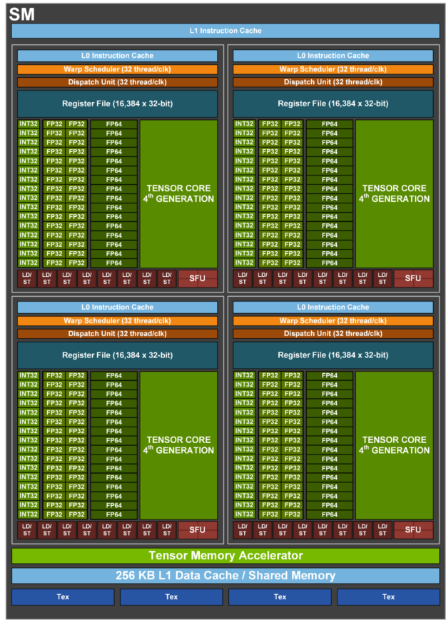
H100 SM key feature summary
- Fourth-generation Tensor Cores:
- Up to 6x faster chip-to-chip compared to A100, including per-SM speedup, additional SM count, and higher clocks of H100.
- On a per SM basis, the Tensor Cores deliver 2x the MMA (Matrix Multiply-Accumulate) computational rates of the A100 SM on equivalent data types, and 4x the rate of A100 using the new FP8 data type, compared to previous generation 16-bit floating point options.
- Sparsity feature exploits fine-grained structured sparsity in deep learning networks, doubling the performance of standard Tensor Core operations
- New DPX instructions accelerate dynamic programming algorithms by up to 7x over the A100 GPU. Two examples include the Smith-Waterman algorithm for genomics processing, and the Floyd-Warshall algorithm used to find optimal routes for a fleet of robots through a dynamic warehouse environment.
- 3x faster IEEE FP64 and FP32 processing rates chip-to-chip compared to A100, due to 2x faster clock-for-clock performance per SM, plus additional SM counts and higher clocks of H100.
- 256 KB of combined shared memory and L1 data cache, 1.33x larger than A100.
- New asynchronous execution features include a new Tensor Memory Accelerator (TMA) unit that can efficiently transfer large blocks of data between global memory and shared memory. TMA also supports asynchronous copies between thread blocks in a cluster. There is also a new asynchronous transaction barrier for doing atomic data movement and synchronization.
- New thread block cluster feature exposes control of locality across multiple SMs.
- Distributed shared memory enables direct SM-to-SM communications for loads, stores, and atomics across multiple SM shared memory blocks
H100 Tensor Core architecture
Tensor Cores are specialized high-performance compute cores for matrix multiply and accumulate (MMA) math operations that provide groundbreaking performance for AI and HPC applications. Tensor Cores operating in parallel across SMs in one NVIDIA GPU deliver massive increases in throughput and efficiency compared to standard floating-point (FP), integer (INT), and fused multiply-accumulate (FMA) operations.
Tensor Cores were first introduced in the NVIDIA V100 GPU, and further enhanced in each new NVIDIA GPU architecture generation.
The new fourth-generation Tensor Core architecture in H100 delivers double the raw dense and sparse matrix math throughput per SM, clock-for-clock, compared to A100, and even more when considering the higher GPU Boost clock of H100 over A100. The FP8, FP16, BF16, TF32, FP64, and INT8 MMA data types are supported. The new Tensor Cores also have more efficient data management, saving up to 30% operand delivery power.
NVIDIA Hopper FP8 data format
The H100 GPU adds FP8 Tensor Cores to accelerate both AI training and inference. As shown in Figure 6, FP8 Tensor Cores support FP32 and FP16 accumulators, and two new FP8 input types:
- E4M3 with 4 exponent bits, 3 mantissa bits, and 1 sign bit
- E5M2, with 5 exponent bits, 2 mantissa bits, and 1 sign bit
E4M3 supports computations requiring less dynamic range with more precision, while E5M2 provides a wider dynamic range and less precision. FP8 halves data storage requirements and doubles throughput compared to FP16 or BF16.
The new transformer engine described later in this post uses both FP8 and FP16 precisions to reduce memory usage and increase performance, while still maintaining accuracy for large language and other models.
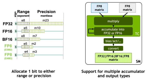
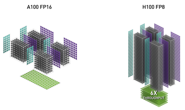
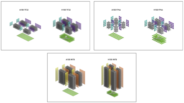
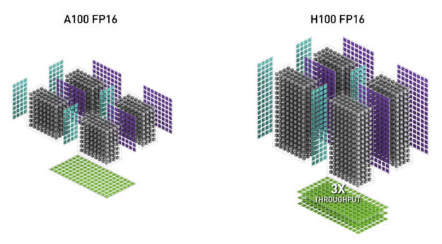
Table 2 shows the H100 math speedups over A100 for multiple data types.
| (measurements in TFLOPS) | A100 | A100 Sparse | H100 SXM51 | H100 SXM51 Sparse | H100 SXM51 Speedup vs A100 |
| FP8 Tensor Core | 2000 | 4000 | 6.4x vs A100 FP16 | ||
| FP16 | 78 | 120 | 1.5x | ||
| FP16 Tensor Core | 312 | 624 | 1000 | 2000 | 3.2x |
| BF16 Tensor Core | 312 | 624 | 1000 | 2000 | 3.2x |
| FP32 | 19.5 | 60 | 3.1x | ||
| TF32 Tensor Core | 156 | 312 | 500 | 1000 | 3.2x |
| FP64 | 9.7 | 30 | 3.1x | ||
| FP64 Tensor Core | 19.5 | 60 | 3.1x | ||
| INT8 Tensor Core | 624 TOPS | 1248 TOPS | 2000 | 4000 | 3.2x |
1 – Preliminary performance estimates for H100 based on current expectations and subject to change in the shipping products
New DPX instructions for accelerated dynamic programming
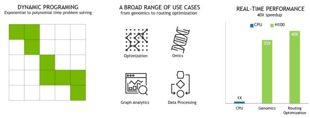
Many brute force optimization algorithms have the property that a sub-problem solution is reused many times when solving the larger problem. Dynamic programming (DP) is an algorithmic technique for solving a complex recursive problem by breaking it down into simpler sub-problems. By storing the results of sub-problems, without the need to recompute them when needed later, DP algorithms reduce the computational complexity of exponential problem sets to a linear scale.
DP is commonly used in a broad range of optimization, data processing, and genomics algorithms.
- In the rapidly growing field of genome sequencing, the Smith-Waterman DP algorithm is one of the most important methods in use.
- In the robotics space, Floyd-Warshall is a key algorithm used to find optimal routes for a fleet of robots through a dynamic warehouse environment in real time.
H100 introduces DPX instructions to accelerate the performance of DP algorithms by up to 7x compared to NVIDIA Ampere GPUs. These new instructions provide support for advanced fused operands for the inner loop of many DP algorithms. This leads to dramatically faster times-to-solution in disease diagnosis, logistics routing optimizations, and even graph analytics.
H100 compute performance summary
Overall, H100 provides approximately 6x compute performance improvement over A100 when factoring in all the new compute technology advances in H100. Figure 10 summarizes the improvements in H100 in a cascading manner:
- 132 SMs provide a 22% SM count increase over the A100 108 SMs
- Each of the H100 SMs is 2x faster, thanks to its new fourth-generation Tensor Core.
- Within each Tensor Core, the new FP8 format and associated transformer engine provide another 2x improvement.
- Increased clock frequencies in H100 deliver another approximately 1.3x performance improvement.
In total, these improvements give H100 approximately 6x the peak compute throughput of A100, a major leap for the world’s most compute-hungry workloads.
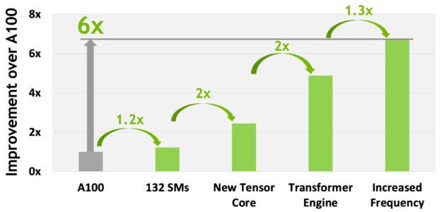
H100 provides 6x throughput for the world’s most compute-hungry workloads.
H100 GPU hierarchy and asynchrony improvements
Two essential keys to achieving high performance in parallel programs are data locality and asynchronous execution. By moving program data as close as possible to the execution units, a programmer can exploit the performance that comes from having lower latency and higher bandwidth access to local data. Asynchronous execution involves finding independent tasks to overlap with memory transfers and other processing. The goal is to keep all the units in the GPU fully used.
In the next section, we explore an important new tier added to the GPU programming hierarchy in NVIDIA Hopper that exposes locality at a scale larger than a single thread block on a single SM. We also describe new asynchronous execution features that improve performance and reduce synchronization overhead.
Thread block clusters
The CUDA programming model has long relied on a GPU compute architecture that uses grids containing multiple thread blocks to leverage locality in a program. A thread block contains multiple threads that run concurrently on a single SM, where the threads can synchronize with fast barriers and exchange data using the SM’s shared memory. However, as GPUs grow beyond 100 SMs, and compute programs become more complex, the thread block as the only unit of locality expressed in the programming model is insufficient to maximize execution efficiency.
H100 introduces a new thread block cluster architecture that exposes control of locality at a granularity larger than a single thread block on a single SM. Thread block clusters extend the CUDA programming model and add another level to the GPU’s physical programming hierarchy to include threads, thread blocks, thread block clusters, and grids.
A cluster is a group of thread blocks that are guaranteed to be concurrently scheduled onto a group of SMs, where the goal is to enable efficient cooperation of threads across multiple SMs. The clusters in H100 run concurrently across SMs within a GPC.
A GPC is a group of SMs in the hardware hierarchy that are always physically close together. Clusters have hardware-accelerated barriers and new memory access collaboration capabilities discussed in the following sections. A dedicated SM-to-SM network for SMs in a GPC provides fast data sharing between threads in a cluster.
In CUDA, thread blocks in a grid can optionally be grouped at kernel launch into clusters as shown in Figure 11, and cluster capabilities can be leveraged from the CUDA cooperative_groups API.
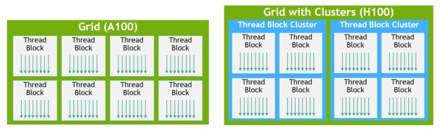
A grid is composed of thread blocks in the legacy CUDA programming model as in A100, shown in the left half of the diagram. The NVIDIA Hopper Architecture adds an optional cluster hierarchy, shown in the right half of the diagram.
Distributed shared memory
With clusters, it is possible for all the threads to directly access other SM’s shared memory with load, store, and atomic operations. This feature is called distributed shared memory (DSMEM) because shared memory virtual address space is logically distributed across all the blocks in the cluster.
DSMEM enables more efficient data exchange between SMs, where data no longer must be written to and read from global memory to pass the data. The dedicated SM-to-SM network for clusters ensures fast, low latency access to remote DSMEM. Compared to using global memory, DSMEM accelerates data exchange between thread blocks by about 7x.
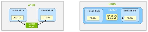
At the CUDA level, all the DSMEM segments from all thread blocks in the cluster are mapped into the generic address space of each thread, such that all DSMEM can be referenced directly with simple pointers. CUDA users can leverage the cooperative_groups API to construct generic pointers to any thread block in the cluster. DSMEM transfers can also be expressed as asynchronous copy operations synchronized with shared memory-based barriers for tracking completion.
Figure 13 shows the performance advantage of using clusters on different algorithms. Clusters improve the performance by enabling you to directly control a larger portion of the GPU than just a single SM. Clusters enable cooperative execution with a larger number of threads, with access to a larger pool of shared memory than is possible with just a single thread block.
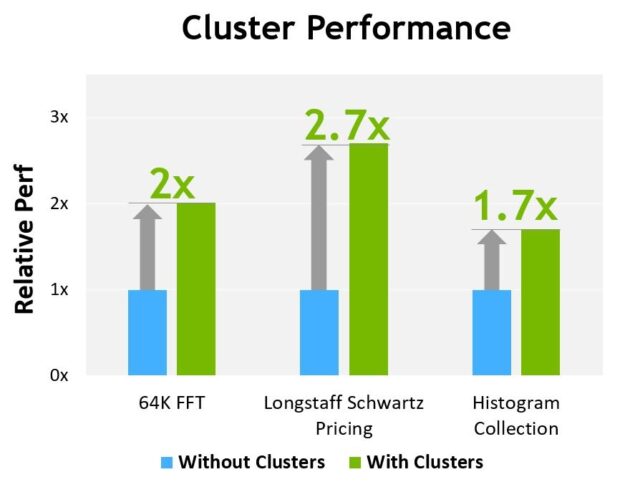
Preliminary performance estimates for H100 based on current expectations and subject to change in the shipping products
Asynchronous execution
Each new generation of NVIDIA GPUs includes numerous architectural enhancements to improve performance, programmability, power efficiency, GPU utilization, and many other factors. Recent NVIDIA GPU generations have included asynchronous execution capabilities to enable more overlap of data movement, computation, and synchronization.
The NVIDIA Hopper Architecture provides new features that improve asynchronous execution and enable further overlap of memory copies with computation and other independent work, while also minimizing synchronization points. We describe the new async memory copy unit called the Tensor Memory Accelerator (TMA) and a new asynchronous transaction barrier.
Programmatic overlap of data movement, computation, and synchronization. Asynchronous concurrency and minimizing synchronization points are keys to performance.
Tensor Memory Accelerator
To help feed the powerful new H100 Tensor Cores, data fetch efficiency is improved with the new Tensor Memory Accelerator (TMA), which can transfer large blocks of data and multidimensional tensors from global memory to shared memory and back again.
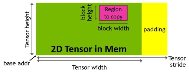
TMA operations are launched using a copy descriptor that specifies data transfers using tensor dimensions and block coordinates instead of per-element addressing (Figure 15). Large blocks of data up to the shared memory capacity can be specified and loaded from global memory into shared memory or stored from shared memory back to global memory. TMA significantly reduces addressing overhead and improves efficiency with support for different tensor layouts (1D-5D tensors), different memory access modes, reductions, and other features.
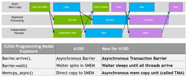
The TMA operation is asynchronous and leverages the shared memory-based asynchronous barriers introduced in A100. Also, the TMA programming model is single-threaded, where a single thread in a warp is elected to issue an asynchronous TMA operation (cuda::memcpy_async) to copy a tensor. As a result, multiple threads can wait on a cuda::barrier for completion of the data transfer. To further improve performance, the H100 SM adds hardware to accelerate these asynchronous-barrier wait operations.
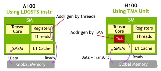
A key advantage of TMA is that it frees the threads to execute other independent work. On A100 (Figure 16, left), asynchronous memory copies were executed using a special LoadGlobalStoreShared instruction, so the threads were responsible for generating all addresses and looping across the whole copy region.
On NVIDIA Hopper, TMA takes care of everything. A single thread creates a copy descriptor before launching the TMA, and from then on address generation and data movement are handled in hardware. TMA provides a much simpler programming model because it takes over the task of computing stride, offset, and boundary calculations when copying segments of a tensor.
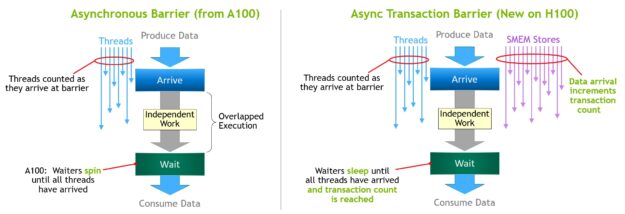
Asynchronous transaction barrier
Asynchronous barriers were originally introduced in the NVIDIA Ampere Architecture (Figure 17, left). Consider an example where a set of threads are producing data that they all consume after a barrier. Asynchronous barriers split the synchronization process into two steps.
- First, threads signal
Arrivewhen they are done producing their portion of the shared data. ThisArriveis non-blocking so that the threads are free to execute other independent work. - Eventually, the threads need the data produced by all the other threads. At this point, they do a
Wait, which blocks them until every thread has signaledArrive.
The advantage of asynchronous barriers is they enable threads that arrive early to execute independent work while waiting. This overlap is the source of extra performance. If there is enough independent work for all threads, the barrier effectively becomes free because the Wait instruction can retire immediately, as all threads have already arrived.
New for NVIDIA Hopper is the ability for waiting threads to sleep until all other threads arrive. On previous chips, waiting threads would spin on the barrier object in shared memory.
While asynchronous barriers are still part of the NVIDIA Hopper programming model, it adds a new form of barrier called an asynchronous transaction barrier. The asynchronous transaction barrier is similar to an asynchronous barrier (Figure 17, right). It too is a split barrier, but instead of counting just thread arrivals, it also counts transactions.
NVIDIA Hopper includes a new command for writing shared memory that passes both the data to be written and a transaction count. The transaction count is essentially a byte count. The asynchronous transaction barrier blocks threads at the Wait command until all the producer threads have performed an Arrive, and the sum of all the transaction counts reaches an expected value.
Asynchronous transaction barriers are a powerful new primitive for async mem copies or data exchanges. As mentioned earlier, clusters can do thread block-to-thread block communication for a data exchange with implied synchronization, and that cluster capability is built on top of asynchronous transaction barriers.
H100 HBM and L2 cache memory architectures
The design of a GPU’s memory architecture and hierarchy is critical to application performance, and affects GPU size, cost, power usage, and programmability. Many memory subsystems exist in a GPU, from the large complement of off-chip DRAM (frame buffer) device memory and varying levels and types of on-chip memories to the register files used in computations in the SM.
H100 HBM3 and HBM2e DRAM subsystems
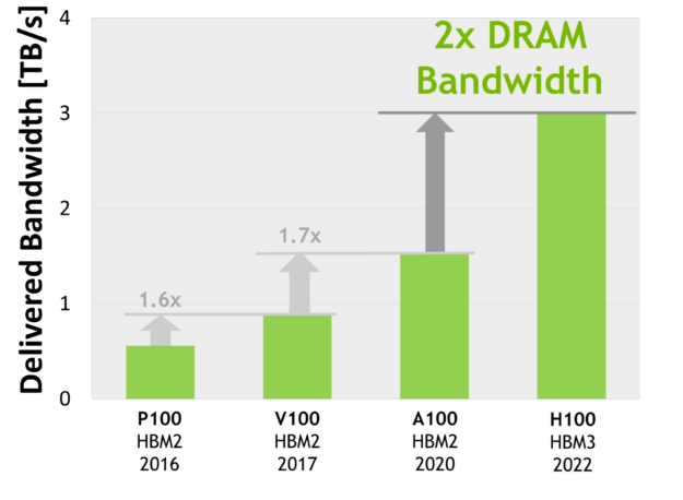
As HPC, AI, and data analytics datasets continue to grow in size, and computing problems get increasingly complex, greater GPU memory capacity and bandwidth is a necessity.
- The NVIDIA P100 was the world’s first GPU architecture to support the high-bandwidth HBM2 memory technology.
- The NVIDIA V100 provided an even faster, more efficient, and higher capacity HBM2 implementation.
- The NVIDIA A100 GPU further increased HBM2 performance and capacity.
The H100 SXM5 GPU raises the bar considerably by supporting 80 GB (five stacks) of fast HBM3 memory, delivering over 3 TB/sec of memory bandwidth, effectively a 2x increase over the memory bandwidth of A100 that was launched just two years ago. The PCIe H100 provides 80 GB of fast HBM2e with over 2 TB/sec of memory bandwidth.
Memory data rates not finalized and subject to change in the final product.
H100 L2 cache
A 50 MB L2 cache in H100 is 1.25x larger than the A100 40 MB L2. It enables caching of even larger portions of models and datasets for repeated access, reducing trips to HBM3 or HBM2e DRAM and improving performance.
Using a partitioned crossbar structure, the L2 cache localizes and caches data for memory accesses from SMs in GPCs directly connected to the partition. L2 cache residency controls optimize capacity utilization, enabling you to selectively manage data that should remain in cache or be evicted.
Both the HBM3 or HBM2e DRAM and L2 cache subsystems support data compression and decompression technology to optimize memory and cache usage and performance.
| GPU Features | NVIDIA A100 | NVIDIA H100 SXM51 | NVIDIA H100 PCIe1 |
| GPU Architecture | NVIDIA Ampere | NVIDIA Hopper | NVIDIA Hopper |
| GPU Board Form Factor | SXM4 | SXM5 | PCIe Gen 5 |
| SMs | 108 | 132 | 114 |
| TPCs | 54 | 62 | 57 |
| FP32 Cores / SM | 64 | 128 | 128 |
| FP32 Cores / GPU | 6912 | 15872 | 14592 |
| FP64 Cores / SM (excl. Tensor) | 32 | 64 | 64 |
| FP64 Cores / GPU (excl. Tensor) | 3456 | 8448 | 7296 |
| INT32 Cores / SM | 64 | 64 | 64 |
| INT32 Cores / GPU | 6912 | 8448 | 7296 |
| Tensor Cores / SM | 4 | 4 | 4 |
| Tensor Cores / GPU | 432 | 528 | 456 |
| GPU Boost Clock (Not finalized for H100)3 |
1410 MHz | Not finalized | Not finalized |
| Peak FP8 Tensor TFLOPS with FP16 Accumulate1 | N/A | 2000/40002 | 1600/32002 |
| Peak FP8 Tensor TFLOPS with FP32 Accumulate1 | N/A | 2000/40002 | 1600/32002 |
| Peak FP16 Tensor TFLOPS with FP16 Accumulate1 | 312/6242 | 1000/20002 | 800/16002 |
| Peak FP16 Tensor TFLOPS with FP32 Accumulate1 | 312/6242 | 1000/20002 | 800/16002 |
| Peak BF16 Tensor TFLOPS with FP32 Accumulate1 | 312/6242 | 1000/20002 | 800/16002 |
| Peak TF32 Tensor TFLOPS1 | 156/3122 | 500/10002 | 400/8002 |
| Peak FP64 Tensor TFLOPS1 | 19.5 | 60 | 48 |
| Peak INT8 Tensor TOPS1 | 624/12482 | 2000/40002 | 1600/32002 |
| Peak FP16 TFLOPS (non-Tensor)1 | 78 | 120 | 96 |
| Peak BF16 TFLOPS (non-Tensor)1 | 39 | 120 | 96 |
| Peak FP32 TFLOPS (non-Tensor)1 | 19.5 | 60 | 48 |
| Peak FP64 TFLOPS (non-Tensor)1 | 9.7 | 30 | 24 |
| Peak INT32 TOPS1 | 19.5 | 30 | 24 |
| Texture Units | 432 | 528 | 456 |
| Memory Interface | 5120-bit HBM2 | 5120-bit HBM3 | 5120-bit HBM2e |
| Memory Size | 40 GB | 80 GB | 80 GB |
| Memory Data Rate (Not finalized for H100)1 |
1215 MHz DDR | Not finalized | Not finalized |
| Memory Bandwidth1 | 1555 GB/sec | 3000 GB/sec | 2000 GB/sec |
| L2 Cache Size | 40 MB | 50 MB | 50 MB |
| Shared Memory Size / SM | Configurable up to 164 KB | Configurable up to 228 KB | Configurable up to 228 KB |
| Register File Size / SM | 256 KB | 256 KB | 256 KB |
| Register File Size / GPU | 27648 KB | 33792 KB | 29184 |
| TDP1 | 400 Watts | 700W | 350W |
| Transistors | 54.2 billion | 80 billion | 80 billion |
| GPU Die Size | 826 mm2 | 814 mm2 | 814 mm2 |
| TSMC Manufacturing Process | 7 nm N7 | 4N customized for NVIDIA | 4N customized for NVIDIA |
- Preliminary specifications for H100 based on current expectations and are subject to change in the shipping products
- Effective TOPS / TFLOPS using the Sparsity feature
- GPU Peak Clock and GPU Boost Clock are synonymous for NVIDIA Data Center GPUs
Because the H100 and A100 Tensor Core GPUs are designed to be installed in high-performance servers and data center racks to power AI and HPC compute workloads, they do not include display connectors, NVIDIA RT Cores for ray-tracing acceleration, or an NVENC encoder.
Compute Capability
The H100 GPU supports the new Compute Capability 9.0. Table 4 compares the parameters of different compute capabilities for NVIDIA GPU architectures.
| Data Center GPU | NVIDIA V100 | NVIDIA A100 | NVIDIA H100 |
| GPU architecture | NVIDIA Volta | NVIDIA Ampere | NVIDIA Hopper |
| Compute capability | 7.0 | 8.0 | 9.0 |
| Threads / warp | 32 | 32 | 32 |
| Max warps / SM | 64 | 64 | 64 |
| Max threads / SM | 2048 | 2048 | 2048 |
| Max thread blocks (CTAs) / SM | 32 | 32 | 32 |
| Max thread blocks / thread block clusters | N/A | N/A | 16 |
| Max 32-bit registers / SM | 65536 | 65536 | 65536 |
| Max registers / thread block (CTA) | 65536 | 65536 | 65536 |
| Max registers / thread | 255 | 255 | 255 |
| Max thread block size (# of threads) | 1024 | 1024 | 1024 |
| FP32 cores / SM | 64 | 64 | 128 |
| Ratio of SM registers to FP32 cores | 1024 | 1024 | 512 |
| Shared memory size / SM | Configurable up to 96 KB | Configurable up to 164 KB | Configurable up to 228 KB |
Transformer engine
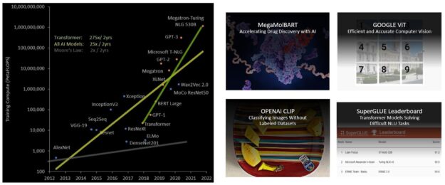
Transformer models are the backbone of language models used widely today from BERT to GPT-3 and they require enormous compute resources. Initially developed for natural language processing (NLP), transformers are increasingly applied across diverse fields such as computer vision, drug discovery, and more.
Their size continues to increase exponentially, now reaching trillions of parameters and causing their training times to stretch into months, which is impractical for business needs due to the large compute requirements . For example, Megatron Turing NLG (MT-NLG) requires 2048 NVIDIA A100 GPUs running for 8 weeks to train. Overall, transformer models have been growing much faster than most other AI models at the rate of 275x every 2 years for the past 5 years (Figure 19).
H100 includes a new transformer engine that uses software and custom NVIDIA Hopper Tensor Core technology to dramatically accelerate the AI calculations for transformers.
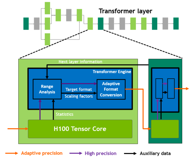
The goal of mixed precision is to manage the precision intelligently to maintain accuracy, while still gaining the performance of smaller, faster numerical formats. At each layer of a transformer model, the transformer engine analyzes the statistics of the output values produced by the Tensor Core.
With knowledge about which type of neural network layer comes next and the precision that it requires, the transformer engine also decides which target format to convert the tensor to before storing it to memory. FP8 has a more limited range than other numerical formats.
To use the available range optimally, the transformer engine also dynamically scales tensor data into the representable range using scaling factors computed from the tensor statistics. Therefore, every layer operates with exactly the range it requires and is accelerated in an optimal manner.
Fourth-generation NVLink and NVLink Network
The emerging class of exascale HPC and trillion-parameter AI models for tasks like superhuman conversational AI require months to train, even on supercomputers. Compressing this extended training time from months to days to be more useful for businesses requires high-speed, seamless communication between every GPU in a server cluster. PCIe creates a bottleneck with its limited bandwidth. To build the most powerful end-to-end computing platform, a faster, more scalable NVLink interconnect is needed.
NVLink is the NVIDIA high-bandwidth, energy-efficient, low-latency, lossless GPU-to-GPU interconnect that includes resiliency features, such as link-level error detection and packet replay mechanisms to guarantee successful transmission of data. The new fourth-generation of NVLink is implemented in H100 GPUs and delivers 1.5x the communications bandwidth compared to the prior third-generation NVLink used in the NVIDIA A100 Tensor Core GPU.
Operating at 900 GB/sec total bandwidth for multi-GPU I/O and shared memory accesses, the new NVLink provides 7x the bandwidth of PCIe Gen 5. The third-generation NVLink in the A100 GPU uses four differential pairs (lanes) in each direction to create a single link delivering 25 GB/sec effective bandwidth in each direction. In contrast, fourth-generation NVLink uses only two high-speed differential pairs in each direction to form a single link, also delivering 25 GB/sec effective bandwidth in each direction.
- H100 includes 18 fourth-generation NVLink links to provide 900 GB/sec total bandwidth.
- A100 includes 12 third-generation NVLink links to provide 600 GB/sec total bandwidth.
On top of fourth-generation NVLink, H100 also introduces the new NVLink Network interconnect, a scalable version of NVLink that enables GPU-to-GPU communication among up to 256 GPUs across multiple compute nodes.
Unlike regular NVLink, where all GPUs share a common address space and requests are routed directly using GPU physical addresses, NVLink Network introduces a new network address space. It is supported by new address translation hardware in H100 to isolate all GPU address spaces from one another and from the network address space. This enables NVLink Network to scale securely to larger numbers of GPUs.
Because NVLink Network endpoints do not share a common memory address space, NVLink Network connections are not automatically established across the entire system. Instead, similar to other networking interfaces such as InfiniBand, the user software should explicitly establish connections between endpoints as needed.
Third-generation NVSwitch
New third-generation NVSwitch technology includes switches residing both inside and outside of nodes to connect multiple GPUs in servers, clusters, and data center environments. Each new third-generation NVSwitch inside a node provides 64 ports of fourth-generation NVLink links to accelerate multi-GPU connectivity. Total switch throughput increases to 13.6 Tbits/sec from 7.2 Tbits/sec in the prior generation.
The new third-generation NVSwitch also provides hardware acceleration of collective operations with multicast and NVIDIA SHARP in-network reductions. Accelerated collectives include write broadcast (all_gather), reduce_scatter, and broadcast atomics. In-fabric multicast and reductions provide up to 2x throughput gain while significantly reducing latency for small block size collectives over using NVIDIA Collective Communications Library (NCCL) on A100. NVSwitch acceleration of collectives significantly reduces the load on SMs for collective communications.
New NVLink Switch System
Combining the new NVLINK Network technology and new third-generation NVSwitch enables NVIDIA to build large scale-up NVLink Switch System networks with unheard-of levels of communication bandwidth. Each GPU node exposes a 2:1 tapered level of all the NVLink bandwidth of the GPUs in the node. The nodes are connected together through a second level of NVSwitches contained in NVLink Switch modules that reside outside of the compute nodes and connect multiple nodes together.
NVLink Switch System supports up to 256 GPUs. The connected nodes can deliver 57.6 TBs of all-to-all bandwidth and can supply an incredible one exaFLOP of FP8 sparse AI compute.
Figure 21 shows a comparison of 32-node, 256 GPU DGX SuperPODs based on A100 versus H100. The H100-based SuperPOD uses the new NVLink Switches to interconnect DGX nodes.
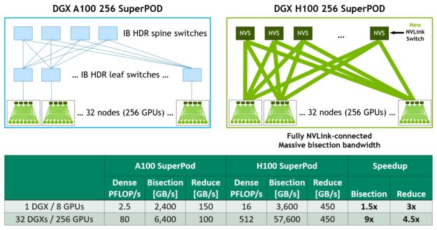
DGX H100 SuperPods can span up to 256 GPUs, fully connected over NVLink Switch System using the new NVLink Switch based on third-generation NVSwitch technology. As the figure shows, compared to an A100-based machine of similar scale with a leaf-spine architecture, no InfiniBand connections are required on the H100 system at all.
The NVLink Network interconnect in 2:1 tapered fat tree topology enables a staggering 9x increase in bisection bandwidth, for example, for all-to-all exchanges, and a 4.5x increase in all-reduce throughput over the previous-generation InfiniBand system.
PCIe Gen 5
H100 incorporates a PCI Express Gen 5 x16 lane interface, providing 128 GB/sec total bandwidth (64 GB/sec in each direction) compared to 64 GB/sec total bandwidth (32GB/sec in each direction) in Gen 4 PCIe included in A100.
Using its PCIe Gen 5 interface, H100 can interface with the highest performing x86 CPUs and SmartNICs and data processing units (DPUs). H100 is designed for optimal connectivity with NVIDIA BlueField-3 DPUs for 400 Gb/s Ethernet or Next Data Rate (NDR) 400 Gb/s InfiniBand networking acceleration for secure HPC and AI workloads.
H100 adds support for native PCIe atomic operations like atomic CAS, atomic exchange, and atomic fetch add for 32-and 64-bit data types, accelerating synchronization and atomic operations between CPU and GPU. H100 also supports single root input/output virtualization (SR-IOV) that enables sharing and virtualizing of a single PCIe-connected GPU for multiple processes or VMs. H100 allows a Virtual Function (VF) or Physical Function (PF) from a single SR-IOV PCIe-connected GPU to access a peer GPU over NVLink.
Summary
For more information about other new and improved H100 features that enhance application performance, see the NVIDIA H100 Tensor Core GPU Architecture whitepaper.
Acknowledgments
We would like to thank Stephen Jones, Manindra Parhy, Atul Kalambur, Harry Petty, Joe DeLaere, Jack Choquette, Mark Hummel, Naveen Cherukuri, Brandon Bell, Jonah Alben, and many other NVIDIA GPU architects and engineers who contributed to this post.
NVIDIA today announced major updates to its NVIDIA AI platform, a suite of software for advancing such workloads as speech, recommender system, hyperscale inference and more, which has been adopted by global industry leaders such as Amazon, Microsoft, Snap and NTT Communications.
When your software can evoke tears of joy, you spread the cheer. So, Translator, a Microsoft Azure Cognitive Service, is applying some of the world’s largest AI models to help more people communicate. “There are so many cool stories,” said Vishal Chowdhary, development manager for Translator. Like the five-day sprint to add Haitian Creole to Read article >
The post Getting People Talking: Microsoft Improves AI Quality and Efficiency of Translator Using NVIDIA Triton appeared first on NVIDIA Blog.
Everyone wants to be heard. And with more people than ever in video calls or live streaming from their home offices, rich audio free from echo hiccups and background noises like barking dogs is key to better sounding online experiences. NVIDIA Maxine offers GPU-accelerated, AI-enabled software development kits to help developers build scalable, low-latency audio Read article >
The post NVIDIA Maxine Reinvents Real-Time Communication With AI appeared first on NVIDIA Blog.
The largest AI models can require months to train on today’s computing platforms. That’s too slow for businesses. AI, high performance computing and data analytics are growing in complexity with some models, like large language ones, reaching trillions of parameters. The NVIDIA Hopper architecture is built from the ground up to accelerate these next-generation AI Read article >
The post H100 Transformer Engine Supercharges AI Training, Delivering Up to 6x Higher Performance Without Losing Accuracy appeared first on NVIDIA Blog.
The NVIDIA Hopper GPU architecture unveiled today at GTC will accelerate dynamic programming — a problem-solving technique used in algorithms for genomics, quantum computing, route optimization and more — by up to 40x with new DPX instructions. An instruction set built into NVIDIA H100 GPUs, DPX will help developers write code to achieve speedups on Read article >
The post NVIDIA Hopper GPU Architecture Accelerates Dynamic Programming Up to 40x Using New DPX Instructions appeared first on NVIDIA Blog.