Categories
Misc

torch time series, take three: Sequence-to-sequence prediction

Today, we continue our exploration of multi-step time-series forecasting with torch. This post is the third in a series.

  • Initially, we covered basics of recurrent neural networks (RNNs), and trained a model to predict the very next value in a sequence. We also found we could forecast quite a few steps ahead by feeding back individual predictions in a loop.

  • Next, we built a model “natively” for multi-step prediction. A small multi-layer-perceptron (MLP) was used to project RNN output to several time points in the future.

Of both approaches, the latter was the more successful. But conceptually, it has an unsatisfying touch to it: When the MLP extrapolates and generates output for, say, ten consecutive points in time, there is no causal relation between those. (Imagine a weather forecast for ten days that never got updated.)

Now, we’d like to try something more intuitively appealing. The input is a sequence; the output is a sequence. In natural language processing (NLP), this type of task is very common: It’s exactly the kind of situation we see with machine translation or summarization.

Quite fittingly, the types of models employed to these ends are named sequence-to-sequence models (often abbreviated seq2seq). In a nutshell, they split up the task into two components: an encoding and a decoding part. The former is done just once per input-target pair. The latter is done in a loop, as in our first try. But the decoder has more information at its disposal: At each iteration, its processing is based on the previous prediction as well as previous state. That previous state will be the encoder’s when a loop is started, and its own ever thereafter.

Before discussing the model in detail, we need to adapt our data input mechanism.

Data input

We continue working with vic_elec , provided by tsibbledata.

Again, the dataset definition in the current post looks a bit different from the way it did before; it’s the shape of the target that differs. This time, y equals x, shifted to the left by one.

The reason we do this is owed to the way we are going to train the network. With seq2seq, people often use a technique called “teacher forcing” where, instead of feeding back its own prediction into the decoder module, you pass it the value it should have predicted. To be clear, this is done during training only, and to a configurable degree.

n_timesteps <- 7 * 24 * 2
n_forecast <- n_timesteps

vic_elec_get_year <- function(year, month = NULL) {
  vic_elec %>%
    filter(year(Date) == year, month(Date) == if (is.null(month)) month(Date) else month) %>%
    as_tibble() %>%
    select(Demand)
}

elec_train <- vic_elec_get_year(2012) %>% as.matrix()
elec_valid <- vic_elec_get_year(2013) %>% as.matrix()
elec_test <- vic_elec_get_year(2014, 1) %>% as.matrix()

train_mean <- mean(elec_train)
train_sd <- sd(elec_train)

elec_dataset <- dataset(
  name = "elec_dataset",
  
  initialize = function(x, n_timesteps, sample_frac = 1) {
    
    self$n_timesteps <- n_timesteps
    self$x <- torch_tensor((x - train_mean) / train_sd)
    
    n <- length(self$x) - self$n_timesteps - 1
    
    self$starts <- sort(sample.int(
      n = n,
      size = n * sample_frac
    ))
    
  },
  
  .getitem = function(i) {
    
    start <- self$starts[i]
    end <- start + self$n_timesteps - 1
    lag <- 1
    
    list(
      x = self$x[start:end],
      y = self$x[(start+lag):(end+lag)]$squeeze(2)
    )
    
  },
  
  .length = function() {
    length(self$starts) 
  }
)

Dataset as well as dataloader instantations then can proceed as before.

batch_size <- 32

train_ds <- elec_dataset(elec_train, n_timesteps, sample_frac = 0.5)
train_dl <- train_ds %>% dataloader(batch_size = batch_size, shuffle = TRUE)

valid_ds <- elec_dataset(elec_valid, n_timesteps, sample_frac = 0.5)
valid_dl <- valid_ds %>% dataloader(batch_size = batch_size)

test_ds <- elec_dataset(elec_test, n_timesteps)
test_dl <- test_ds %>% dataloader(batch_size = 1)

Model

Technically, the model consists of three modules: the aforementioned encoder and decoder, and the seq2seq module that orchestrates them.

Encoder

The encoder takes its input and runs it through an RNN. Of the two things returned by a recurrent neural network, outputs and state, so far we’ve only been using output. This time, we do the opposite: We throw away the outputs, and only return the state.

If the RNN in question is a GRU (and assuming that of the outputs, we take just the final time step, which is what we’ve been doing throughout), there really is no difference: The final state equals the final output. If it’s an LSTM, however, there is a second kind of state, the “cell state”. In that case, returning the state instead of the final output will carry more information.

encoder_module <- nn_module(
  
  initialize = function(type, input_size, hidden_size, num_layers = 1, dropout = 0) {
    
    self$type <- type
    
    self$rnn <- if (self$type == "gru") {
      nn_gru(
        input_size = input_size,
        hidden_size = hidden_size,
        num_layers = num_layers,
        dropout = dropout,
        batch_first = TRUE
      )
    } else {
      nn_lstm(
        input_size = input_size,
        hidden_size = hidden_size,
        num_layers = num_layers,
        dropout = dropout,
        batch_first = TRUE
      )
    }
    
  },
  
  forward = function(x) {
    
    x <- self$rnn(x)
    
    # return last states for all layers
    # per layer, a single tensor for GRU, a list of 2 tensors for LSTM
    x <- x[[2]]
    x
    
  }
  
)

Decoder

In the decoder, just like in the encoder, the main component is an RNN. In contrast to previously-shown architectures, though, it does not just return a prediction. It also reports back the RNN’s final state.

decoder_module <- nn_module(
  
  initialize = function(type, input_size, hidden_size, num_layers = 1) {
    
    self$type <- type
    
    self$rnn <- if (self$type == "gru") {
      nn_gru(
        input_size = input_size,
        hidden_size = hidden_size,
        num_layers = num_layers,
        batch_first = TRUE
      )
    } else {
      nn_lstm(
        input_size = input_size,
        hidden_size = hidden_size,
        num_layers = num_layers,
        batch_first = TRUE
      )
    }
    
    self$linear <- nn_linear(hidden_size, 1)
    
  },
  
  forward = function(x, state) {
    
    # input to forward:
    # x is (batch_size, 1, 1)
    # state is (1, batch_size, hidden_size)
    x <- self$rnn(x, state)
    
    # break up RNN return values
    # output is (batch_size, 1, hidden_size)
    # next_hidden is
    c(output, next_hidden) %<-% x
    
    output <- output$squeeze(2)
    output <- self$linear(output)
    
    list(output, next_hidden)
    
  }
  
)

seq2seq module

seq2seq is where the action happens. The plan is to encode once, then call the decoder in a loop.

If you look back to decoder forward(), you see that it takes two arguments: x and state.

Depending on the context, x corresponds to one of three things: final input, preceding prediction, or prior ground truth.

  • The very first time the decoder is called on an input sequence, x maps to the final input value. This is different from a task like machine translation, where you would pass in a start token. With time series, though, we’d like to continue where the actual measurements stop.

  • In further calls, we want the decoder to continue from its most recent prediction. It is only logical, thus, to pass back the preceding forecast.

  • That said, in NLP a technique called “teacher forcing” is commonly used to speed up training. With teacher forcing, instead of the forecast we pass the actual ground truth, the thing the decoder should have predicted. We do that only in a configurable fraction of cases, and – naturally – only while training. The rationale behind this technique is that without this form of re-calibration, consecutive prediction errors can quickly erase any remaining signal.

state, too, is polyvalent. But here, there are just two possibilities: encoder state and decoder state.

  • The first time the decoder is called, it is “seeded” with the final state from the encoder. Note how this is the only time we make use of the encoding.

  • From then on, the decoder’s own previous state will be passed. Remember how it returns two values, forecast and state?

seq2seq_module <- nn_module(
  
  initialize = function(type, input_size, hidden_size, n_forecast, num_layers = 1, encoder_dropout = 0) {
    
    self$encoder <- encoder_module(type = type, input_size = input_size,
                                   hidden_size = hidden_size, num_layers, encoder_dropout)
    self$decoder <- decoder_module(type = type, input_size = input_size,
                                   hidden_size = hidden_size, num_layers)
    self$n_forecast <- n_forecast
    
  },
  
  forward = function(x, y, teacher_forcing_ratio) {
    
    # prepare empty output
    outputs <- torch_zeros(dim(x)[1], self$n_forecast)$to(device = device)
    
    # encode current input sequence
    hidden <- self$encoder(x)
    
    # prime decoder with final input value and hidden state from the encoder
    out <- self$decoder(x[ , n_timesteps, , drop = FALSE], hidden)
    
    # decompose into predictions and decoder state
    # pred is (batch_size, 1)
    # state is (1, batch_size, hidden_size)
    c(pred, state) %<-% out
    
    # store first prediction
    outputs[ , 1] <- pred$squeeze(2)
    
    # iterate to generate remaining forecasts
    for (t in 2:self$n_forecast) {
      
      # call decoder on either ground truth or previous prediction, plus previous decoder state
      teacher_forcing <- runif(1) < teacher_forcing_ratio
      input <- if (teacher_forcing == TRUE) y[ , t - 1, drop = FALSE] else pred
      input <- input$unsqueeze(3)
      out <- self$decoder(input, state)
      
      # again, decompose decoder return values
      c(pred, state) %<-% out
      # and store current prediction
      outputs[ , t] <- pred$squeeze(2)
    }
    outputs
  }
  
)

net <- seq2seq_module("gru", input_size = 1, hidden_size = 32, n_forecast = n_forecast)

# training RNNs on the GPU currently prints a warning that may clutter 
# the console
# see https://github.com/mlverse/torch/issues/461
# alternatively, use 
# device <- "cpu"
device <- torch_device(if (cuda_is_available()) "cuda" else "cpu")

net <- net$to(device = device)

Training

The training procedure is mainly unchanged. We do, however, need to decide about teacher_forcing_ratio, the proportion of input sequences we want to perform re-calibration on. In valid_batch(), this should always be 0, while in train_batch(), it’s up to us (or rather, experimentation). Here, we set it to 0.3.

optimizer <- optim_adam(net$parameters, lr = 0.001)

num_epochs <- 50

train_batch <- function(b, teacher_forcing_ratio) {
  
  optimizer$zero_grad()
  output <- net(b$x$to(device = device), b$y$to(device = device), teacher_forcing_ratio)
  target <- b$y$to(device = device)
  
  loss <- nnf_mse_loss(output, target)
  loss$backward()
  optimizer$step()
  
  loss$item()
  
}

valid_batch <- function(b, teacher_forcing_ratio = 0) {
  
  output <- net(b$x$to(device = device), b$y$to(device = device), teacher_forcing_ratio)
  target <- b$y$to(device = device)
  
  loss <- nnf_mse_loss(output, target)
  
  loss$item()
  
}

for (epoch in 1:num_epochs) {
  
  net$train()
  train_loss <- c()
  
  coro::loop(for (b in train_dl) {
    loss <-train_batch(b, teacher_forcing_ratio = 0.3)
    train_loss <- c(train_loss, loss)
  })
  
  cat(sprintf("nEpoch %d, training: loss: %3.5f n", epoch, mean(train_loss)))
  
  net$eval()
  valid_loss <- c()
  
  coro::loop(for (b in valid_dl) {
    loss <- valid_batch(b)
    valid_loss <- c(valid_loss, loss)
  })
  
  cat(sprintf("nEpoch %d, validation: loss: %3.5f n", epoch, mean(valid_loss)))
}
Epoch 1, training: loss: 0.37961 

Epoch 1, validation: loss: 1.10699 

Epoch 2, training: loss: 0.19355 

Epoch 2, validation: loss: 1.26462 

# ...
# ...

Epoch 49, training: loss: 0.03233 

Epoch 49, validation: loss: 0.62286 

Epoch 50, training: loss: 0.03091 

Epoch 50, validation: loss: 0.54457

It’s interesting to compare performances for different settings of teacher_forcing_ratio. With a setting of 0.5, training loss decreases a lot more slowly; the opposite is seen with a setting of 0. Validation loss, however, is not affected significantly.

Evaluation

The code to inspect test-set forecasts is unchanged.

net$eval()

test_preds <- vector(mode = "list", length = length(test_dl))

i <- 1

coro::loop(for (b in test_dl) {
  
  input <- b$x
  output <- net(input$to(device = device))
  preds <- as.numeric(output)
  
  test_preds[[i]] <- preds
  i <<- i + 1
  
})

vic_elec_jan_2014 <- vic_elec %>%
  filter(year(Date) == 2014, month(Date) == 1)

test_pred1 <- test_preds[[1]]
test_pred1 <- c(rep(NA, n_timesteps), test_pred1, rep(NA, nrow(vic_elec_jan_2014) - n_timesteps - n_forecast))

test_pred2 <- test_preds[[408]]
test_pred2 <- c(rep(NA, n_timesteps + 407), test_pred2, rep(NA, nrow(vic_elec_jan_2014) - 407 - n_timesteps - n_forecast))

test_pred3 <- test_preds[[817]]
test_pred3 <- c(rep(NA, nrow(vic_elec_jan_2014) - n_forecast), test_pred3)


preds_ts <- vic_elec_jan_2014 %>%
  select(Demand) %>%
  add_column(
    mlp_ex_1 = test_pred1 * train_sd + train_mean,
    mlp_ex_2 = test_pred2 * train_sd + train_mean,
    mlp_ex_3 = test_pred3 * train_sd + train_mean) %>%
  pivot_longer(-Time) %>%
  update_tsibble(key = name)


preds_ts %>%
  autoplot() +
  scale_colour_manual(values = c("#08c5d1", "#00353f", "#ffbf66", "#d46f4d")) +
  theme_minimal()
One-week-ahead predictions for January, 2014.

(#fig:unnamed-chunk-8)One-week-ahead predictions for January, 2014.

Comparing this to the forecast obtained from last time’s RNN-MLP combo, we don’t see much of a difference. Is this surprising? To me it is. If asked to speculate about the reason, I would probably say this: In all of the architectures we’ve used so far, the main carrier of information has been the final hidden state of the RNN (one and only RNN in the two previous setups, encoder RNN in this one). It will be interesting to see what happens in the last part of this series, when we augment the encoder-decoder architecture by attention.

Thanks for reading!

Photo by Suzuha Kozuki on Unsplash

Categories
Offsites

torch time series, take three: Sequence-to-sequence prediction

Today, we continue our exploration of multi-step time-series forecasting with torch. This post is the third in a series.

  • Initially, we covered basics of recurrent neural networks (RNNs), and trained a model to predict the very next value in a sequence. We also found we could forecast quite a few steps ahead by feeding back individual predictions in a loop.

  • Next, we built a model “natively” for multi-step prediction. A small multi-layer-perceptron (MLP) was used to project RNN output to several time points in the future.

Of both approaches, the latter was the more successful. But conceptually, it has an unsatisfying touch to it: When the MLP extrapolates and generates output for, say, ten consecutive points in time, there is no causal relation between those. (Imagine a weather forecast for ten days that never got updated.)

Now, we’d like to try something more intuitively appealing. The input is a sequence; the output is a sequence. In natural language processing (NLP), this type of task is very common: It’s exactly the kind of situation we see with machine translation or summarization.

Quite fittingly, the types of models employed to these ends are named sequence-to-sequence models (often abbreviated seq2seq). In a nutshell, they split up the task into two components: an encoding and a decoding part. The former is done just once per input-target pair. The latter is done in a loop, as in our first try. But the decoder has more information at its disposal: At each iteration, its processing is based on the previous prediction as well as previous state. That previous state will be the encoder’s when a loop is started, and its own ever thereafter.

Before discussing the model in detail, we need to adapt our data input mechanism.

Data input

We continue working with vic_elec , provided by tsibbledata.

Again, the dataset definition in the current post looks a bit different from the way it did before; it’s the shape of the target that differs. This time, y equals x, shifted to the left by one.

The reason we do this is owed to the way we are going to train the network. With seq2seq, people often use a technique called “teacher forcing” where, instead of feeding back its own prediction into the decoder module, you pass it the value it should have predicted. To be clear, this is done during training only, and to a configurable degree.

n_timesteps <- 7 * 24 * 2
n_forecast <- n_timesteps

vic_elec_get_year <- function(year, month = NULL) {
  vic_elec %>%
    filter(year(Date) == year, month(Date) == if (is.null(month)) month(Date) else month) %>%
    as_tibble() %>%
    select(Demand)
}

elec_train <- vic_elec_get_year(2012) %>% as.matrix()
elec_valid <- vic_elec_get_year(2013) %>% as.matrix()
elec_test <- vic_elec_get_year(2014, 1) %>% as.matrix()

train_mean <- mean(elec_train)
train_sd <- sd(elec_train)

elec_dataset <- dataset(
  name = "elec_dataset",
  
  initialize = function(x, n_timesteps, sample_frac = 1) {
    
    self$n_timesteps <- n_timesteps
    self$x <- torch_tensor((x - train_mean) / train_sd)
    
    n <- length(self$x) - self$n_timesteps - 1
    
    self$starts <- sort(sample.int(
      n = n,
      size = n * sample_frac
    ))
    
  },
  
  .getitem = function(i) {
    
    start <- self$starts[i]
    end <- start + self$n_timesteps - 1
    lag <- 1
    
    list(
      x = self$x[start:end],
      y = self$x[(start+lag):(end+lag)]$squeeze(2)
    )
    
  },
  
  .length = function() {
    length(self$starts) 
  }
)

Dataset as well as dataloader instantations then can proceed as before.

batch_size <- 32

train_ds <- elec_dataset(elec_train, n_timesteps, sample_frac = 0.5)
train_dl <- train_ds %>% dataloader(batch_size = batch_size, shuffle = TRUE)

valid_ds <- elec_dataset(elec_valid, n_timesteps, sample_frac = 0.5)
valid_dl <- valid_ds %>% dataloader(batch_size = batch_size)

test_ds <- elec_dataset(elec_test, n_timesteps)
test_dl <- test_ds %>% dataloader(batch_size = 1)

Model

Technically, the model consists of three modules: the aforementioned encoder and decoder, and the seq2seq module that orchestrates them.

Encoder

The encoder takes its input and runs it through an RNN. Of the two things returned by a recurrent neural network, outputs and state, so far we’ve only been using output. This time, we do the opposite: We throw away the outputs, and only return the state.

If the RNN in question is a GRU (and assuming that of the outputs, we take just the final time step, which is what we’ve been doing throughout), there really is no difference: The final state equals the final output. If it’s an LSTM, however, there is a second kind of state, the “cell state”. In that case, returning the state instead of the final output will carry more information.

encoder_module <- nn_module(
  
  initialize = function(type, input_size, hidden_size, num_layers = 1, dropout = 0) {
    
    self$type <- type
    
    self$rnn <- if (self$type == "gru") {
      nn_gru(
        input_size = input_size,
        hidden_size = hidden_size,
        num_layers = num_layers,
        dropout = dropout,
        batch_first = TRUE
      )
    } else {
      nn_lstm(
        input_size = input_size,
        hidden_size = hidden_size,
        num_layers = num_layers,
        dropout = dropout,
        batch_first = TRUE
      )
    }
    
  },
  
  forward = function(x) {
    
    x <- self$rnn(x)
    
    # return last states for all layers
    # per layer, a single tensor for GRU, a list of 2 tensors for LSTM
    x <- x[[2]]
    x
    
  }
  
)

Decoder

In the decoder, just like in the encoder, the main component is an RNN. In contrast to previously-shown architectures, though, it does not just return a prediction. It also reports back the RNN’s final state.

decoder_module <- nn_module(
  
  initialize = function(type, input_size, hidden_size, num_layers = 1) {
    
    self$type <- type
    
    self$rnn <- if (self$type == "gru") {
      nn_gru(
        input_size = input_size,
        hidden_size = hidden_size,
        num_layers = num_layers,
        batch_first = TRUE
      )
    } else {
      nn_lstm(
        input_size = input_size,
        hidden_size = hidden_size,
        num_layers = num_layers,
        batch_first = TRUE
      )
    }
    
    self$linear <- nn_linear(hidden_size, 1)
    
  },
  
  forward = function(x, state) {
    
    # input to forward:
    # x is (batch_size, 1, 1)
    # state is (1, batch_size, hidden_size)
    x <- self$rnn(x, state)
    
    # break up RNN return values
    # output is (batch_size, 1, hidden_size)
    # next_hidden is
    c(output, next_hidden) %<-% x
    
    output <- output$squeeze(2)
    output <- self$linear(output)
    
    list(output, next_hidden)
    
  }
  
)

seq2seq module

seq2seq is where the action happens. The plan is to encode once, then call the decoder in a loop.

If you look back to decoder forward(), you see that it takes two arguments: x and state.

Depending on the context, x corresponds to one of three things: final input, preceding prediction, or prior ground truth.

  • The very first time the decoder is called on an input sequence, x maps to the final input value. This is different from a task like machine translation, where you would pass in a start token. With time series, though, we’d like to continue where the actual measurements stop.

  • In further calls, we want the decoder to continue from its most recent prediction. It is only logical, thus, to pass back the preceding forecast.

  • That said, in NLP a technique called “teacher forcing” is commonly used to speed up training. With teacher forcing, instead of the forecast we pass the actual ground truth, the thing the decoder should have predicted. We do that only in a configurable fraction of cases, and – naturally – only while training. The rationale behind this technique is that without this form of re-calibration, consecutive prediction errors can quickly erase any remaining signal.

state, too, is polyvalent. But here, there are just two possibilities: encoder state and decoder state.

  • The first time the decoder is called, it is “seeded” with the final state from the encoder. Note how this is the only time we make use of the encoding.

  • From then on, the decoder’s own previous state will be passed. Remember how it returns two values, forecast and state?

seq2seq_module <- nn_module(
  
  initialize = function(type, input_size, hidden_size, n_forecast, num_layers = 1, encoder_dropout = 0) {
    
    self$encoder <- encoder_module(type = type, input_size = input_size,
                                   hidden_size = hidden_size, num_layers, encoder_dropout)
    self$decoder <- decoder_module(type = type, input_size = input_size,
                                   hidden_size = hidden_size, num_layers)
    self$n_forecast <- n_forecast
    
  },
  
  forward = function(x, y, teacher_forcing_ratio) {
    
    # prepare empty output
    outputs <- torch_zeros(dim(x)[1], self$n_forecast)$to(device = device)
    
    # encode current input sequence
    hidden <- self$encoder(x)
    
    # prime decoder with final input value and hidden state from the encoder
    out <- self$decoder(x[ , n_timesteps, , drop = FALSE], hidden)
    
    # decompose into predictions and decoder state
    # pred is (batch_size, 1)
    # state is (1, batch_size, hidden_size)
    c(pred, state) %<-% out
    
    # store first prediction
    outputs[ , 1] <- pred$squeeze(2)
    
    # iterate to generate remaining forecasts
    for (t in 2:self$n_forecast) {
      
      # call decoder on either ground truth or previous prediction, plus previous decoder state
      teacher_forcing <- runif(1) < teacher_forcing_ratio
      input <- if (teacher_forcing == TRUE) y[ , t - 1, drop = FALSE] else pred
      input <- input$unsqueeze(3)
      out <- self$decoder(input, state)
      
      # again, decompose decoder return values
      c(pred, state) %<-% out
      # and store current prediction
      outputs[ , t] <- pred$squeeze(2)
    }
    outputs
  }
  
)

net <- seq2seq_module("gru", input_size = 1, hidden_size = 32, n_forecast = n_forecast)

# training RNNs on the GPU currently prints a warning that may clutter 
# the console
# see https://github.com/mlverse/torch/issues/461
# alternatively, use 
# device <- "cpu"
device <- torch_device(if (cuda_is_available()) "cuda" else "cpu")

net <- net$to(device = device)

Training

The training procedure is mainly unchanged. We do, however, need to decide about teacher_forcing_ratio, the proportion of input sequences we want to perform re-calibration on. In valid_batch(), this should always be 0, while in train_batch(), it’s up to us (or rather, experimentation). Here, we set it to 0.3.

optimizer <- optim_adam(net$parameters, lr = 0.001)

num_epochs <- 50

train_batch <- function(b, teacher_forcing_ratio) {
  
  optimizer$zero_grad()
  output <- net(b$x$to(device = device), b$y$to(device = device), teacher_forcing_ratio)
  target <- b$y$to(device = device)
  
  loss <- nnf_mse_loss(output, target)
  loss$backward()
  optimizer$step()
  
  loss$item()
  
}

valid_batch <- function(b, teacher_forcing_ratio = 0) {
  
  output <- net(b$x$to(device = device), b$y$to(device = device), teacher_forcing_ratio)
  target <- b$y$to(device = device)
  
  loss <- nnf_mse_loss(output, target)
  
  loss$item()
  
}

for (epoch in 1:num_epochs) {
  
  net$train()
  train_loss <- c()
  
  coro::loop(for (b in train_dl) {
    loss <-train_batch(b, teacher_forcing_ratio = 0.3)
    train_loss <- c(train_loss, loss)
  })
  
  cat(sprintf("nEpoch %d, training: loss: %3.5f n", epoch, mean(train_loss)))
  
  net$eval()
  valid_loss <- c()
  
  coro::loop(for (b in valid_dl) {
    loss <- valid_batch(b)
    valid_loss <- c(valid_loss, loss)
  })
  
  cat(sprintf("nEpoch %d, validation: loss: %3.5f n", epoch, mean(valid_loss)))
}
Epoch 1, training: loss: 0.37961 

Epoch 1, validation: loss: 1.10699 

Epoch 2, training: loss: 0.19355 

Epoch 2, validation: loss: 1.26462 

# ...
# ...

Epoch 49, training: loss: 0.03233 

Epoch 49, validation: loss: 0.62286 

Epoch 50, training: loss: 0.03091 

Epoch 50, validation: loss: 0.54457

It’s interesting to compare performances for different settings of teacher_forcing_ratio. With a setting of 0.5, training loss decreases a lot more slowly; the opposite is seen with a setting of 0. Validation loss, however, is not affected significantly.

Evaluation

The code to inspect test-set forecasts is unchanged.

net$eval()

test_preds <- vector(mode = "list", length = length(test_dl))

i <- 1

coro::loop(for (b in test_dl) {
  
  input <- b$x
  output <- net(input$to(device = device))
  preds <- as.numeric(output)
  
  test_preds[[i]] <- preds
  i <<- i + 1
  
})

vic_elec_jan_2014 <- vic_elec %>%
  filter(year(Date) == 2014, month(Date) == 1)

test_pred1 <- test_preds[[1]]
test_pred1 <- c(rep(NA, n_timesteps), test_pred1, rep(NA, nrow(vic_elec_jan_2014) - n_timesteps - n_forecast))

test_pred2 <- test_preds[[408]]
test_pred2 <- c(rep(NA, n_timesteps + 407), test_pred2, rep(NA, nrow(vic_elec_jan_2014) - 407 - n_timesteps - n_forecast))

test_pred3 <- test_preds[[817]]
test_pred3 <- c(rep(NA, nrow(vic_elec_jan_2014) - n_forecast), test_pred3)


preds_ts <- vic_elec_jan_2014 %>%
  select(Demand) %>%
  add_column(
    mlp_ex_1 = test_pred1 * train_sd + train_mean,
    mlp_ex_2 = test_pred2 * train_sd + train_mean,
    mlp_ex_3 = test_pred3 * train_sd + train_mean) %>%
  pivot_longer(-Time) %>%
  update_tsibble(key = name)


preds_ts %>%
  autoplot() +
  scale_colour_manual(values = c("#08c5d1", "#00353f", "#ffbf66", "#d46f4d")) +
  theme_minimal()
One-week-ahead predictions for January, 2014.

(#fig:unnamed-chunk-8)One-week-ahead predictions for January, 2014.

Comparing this to the forecast obtained from last time’s RNN-MLP combo, we don’t see much of a difference. Is this surprising? To me it is. If asked to speculate about the reason, I would probably say this: In all of the architectures we’ve used so far, the main carrier of information has been the final hidden state of the RNN (one and only RNN in the two previous setups, encoder RNN in this one). It will be interesting to see what happens in the last part of this series, when we augment the encoder-decoder architecture by attention.

Thanks for reading!

Photo by Suzuha Kozuki on Unsplash

Categories
Misc

Antarctic Observatory Data, Ray Tracing Advance Astrophysics Research

Scientists from the Wisconsin IceCube Particle Astrophysics Center are using ray tracing on NVIDIA GPUs to accelerate simulations of subatomic particles by hundreds of times.

Scientists from the Wisconsin IceCube Particle Astrophysics Center are using ray tracing on NVIDIA GPUs to accelerate simulations of subatomic particles by hundreds of times. 
Using NVIDIA RTX GPUs in a subsystem of the Texas Advanced Computing Center’s Frontera supercomputer, the researchers can calculate the path of light as it travels through a one cubic kilometer block of ice at Antarctica’s IceCube Neutrino Observatory. 

They’re analyzing neutrinos, tiny particles created by cosmic rays that interact with Earth’s atmosphere. The ice block, located at the Amundsen-Scott South Pole Station, is rigged with sensors over a thousand feet under the surface, which transform signals from neutrino interactions into digital data. 

“Based on the analysis, researchers are also able to determine where in the sky the particle came from, its energy, and sometimes, what type of neutrino — electron, muon or tau — it was,” said James Madson, executive director at IceCube.

The researchers are especially interested in neutrino events, or spikes in activity that can be traced to high-energy cosmic events billions of light years away. But these analyses require significant computational resources, making the IceCube team among the largest users of the Frontera GPU subsystem. 

To better understand how neutrinos travel through the observatory’s ice block, the scientists use GPU-accelerated ray tracing to simulate how light propagates through the ice, tracking high-energy particles that are produced when neutrinos interact. Defects in the ice can cause the light to scatter or be absorbed, making it harder to analyze. 

“Large scale simulations of the IceCube facility and the data it creates allow us to rapidly and accurately determine the properties of these neutrinos, which in turn exposes the physics of the most energetic events in the universe,” said Niall Gaffney, director of data intensive computing at the Texas Advanced Computing Center. “This is key to validating the fundamental quantum-mechanical physics in environments that cannot be practically replicated on earth.”

Read more from the Texas Advanced Computing Center >>

Categories
Offsites

Contactless Sleep Sensing in Nest Hub

People often turn to technology to manage their health and wellbeing, whether it is to record their daily exercise, measure their heart rate, or increasingly, to understand their sleep patterns. Sleep is foundational to a person’s everyday wellbeing and can be impacted by (and in turn, have an impact on) other aspects of one’s life — mood, energy, diet, productivity, and more.

As part of our ongoing efforts to support people’s health and happiness, today we announced Sleep Sensing in the new Nest Hub, which uses radar-based sleep tracking in addition to an algorithm for cough and snore detection. While not intended for medical purposes1, Sleep Sensing is an opt-in feature that can help users better understand their nighttime wellness using a contactless bedside setup. Here we describe the technologies behind Sleep Sensing and discuss how we leverage on-device signal processing to enable sleep monitoring (comparable to other clinical- and consumer-grade devices) in a way that protects user privacy.

Soli for Sleep Tracking
Sleep Sensing in Nest Hub demonstrates the first wellness application of Soli, a miniature radar sensor that can be used for gesture sensing at various scales, from a finger tap to movements of a person’s body. In Pixel 4, Soli powers Motion Sense, enabling touchless interactions with the phone to skip songs, snooze alarms, and silence phone calls. We extended this technology and developed an embedded Soli-based algorithm that could be implemented in Nest Hub for sleep tracking.

Soli consists of a millimeter-wave frequency-modulated continuous wave (FMCW) radar transceiver that emits an ultra-low power radio wave and measures the reflected signal from the scene of interest. The frequency spectrum of the reflected signal contains an aggregate representation of the distance and velocity of objects within the scene. This signal can be processed to isolate a specified range of interest, such as a user’s sleeping area, and to detect and characterize a wide range of motions within this region, ranging from large body movements to sub-centimeter respiration.

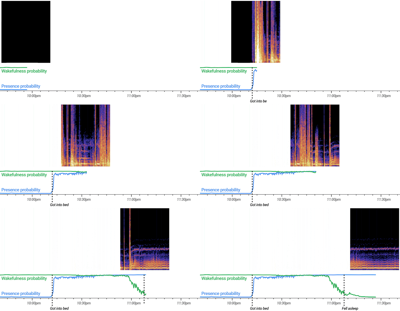
Soli spectrogram illustrating its ability to detect a wide range of motions, characterized as (a) an empty room (no variation in the reflected signal demonstrated by the black space), (b) large pose changes, (c) brief limb movements, and (d) sub-centimeter chest and torso displacements from respiration while at rest.

In order to make use of this signal for Sleep Sensing, it was necessary to design an algorithm that could determine whether a person is present in the specified sleeping area and, if so, whether the person is asleep or awake. We designed a custom machine-learning (ML) model to efficiently process a continuous stream of 3D radar tensors (summarizing activity over a range of distances, frequencies, and time) and automatically classify each feature into one of three possible states: absent, awake, and asleep.

To train and evaluate the model, we recorded more than a million hours of radar data from thousands of individuals, along with thousands of sleep diaries, reference sensor recordings, and external annotations. We then leveraged the TensorFlow Extended framework to construct a training pipeline to process this data and produce an efficient TensorFlow Lite embedded model. In addition, we created an automatic calibration algorithm that runs during setup to configure the part of the scene on which the classifier will focus. This ensures that the algorithm ignores motion from a person on the other side of the bed or from other areas of the room, such as ceiling fans and swaying curtains.

The custom ML model efficiently processes a continuous stream of 3D radar tensors (summarizing activity over a range of distances, frequencies, and time) to automatically compute probabilities for the likelihood of user presence and wakefulness (awake or asleep).

To validate the accuracy of the algorithm, we compared it to the gold-standard of sleep-wake determination, the polysomnogram sleep study, in a cohort of 33 “healthy sleepers” (those without significant sleep issues, like sleep apnea or insomnia) across a broad age range (19-78 years of age). Sleep studies are typically conducted in clinical and research laboratories in order to collect various body signals (brain waves, muscle activity, respiratory and heart rate measurements, body movement and position, and snoring), which can then be interpreted by trained sleep experts to determine stages of sleep and identify relevant events. To account for variability in how different scorers apply the American Academy of Sleep Medicine’s staging and scoring rules, our study used two board-certified sleep technologists to independently annotate each night of sleep and establish a definitive groundtruth.

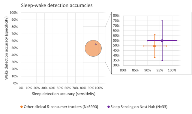
We compared our Sleep Sensing algorithm’s outputs to the corresponding groundtruth sleep and wake labels for every 30-second epoch of time to compute standard performance metrics (e.g., sensitivity and specificity). While not a true head-to-head comparison, this study’s results can be compared against previously published studies in similar cohorts with comparable methodologies in order to get a rough estimate of performance. In “Sleep-wake detection with a contactless, bedside radar sleep sensing system”, we share the full details of these validation results, demonstrating sleep-wake estimation equivalent to or, in some cases, better than current clinical and consumer sleep tracking devices.

Aggregate performance from previously published accuracies for detection of sleep (sensitivity) and wake (specificity) of a variety of sleep trackers against polysomnography in a variety of different studies, accounting for 3,990 nights in total. While this is not a head-to-head comparison, the performance of Sleep Sensing on Nest Hub in a population of healthy sleepers who simultaneously underwent polysomnography is added to the figure for rough comparison. The size of each circle is a reflection of the number of nights and the inset illustrates the mean±standard deviation for the performance metrics.

Understanding Sleep Quality with Audio Sensing
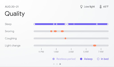
The Soli-based sleep tracking algorithm described above gives users a convenient and reliable way to see how much sleep they are getting and when sleep disruptions occur. However, to understand and improve their sleep, users also need to understand why their sleep is disrupted. To assist with this, Nest Hub uses its array of sensors to track common sleep disturbances, such as light level changes or uncomfortable room temperature. In addition to these, respiratory events like coughing and snoring are also frequent sources of disturbance, but people are often unaware of these events.

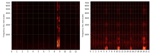
As with other audio-processing applications like speech or music recognition, coughing and snoring exhibit distinctive temporal patterns in the audio frequency spectrum, and with sufficient data an ML model can be trained to reliably recognize these patterns while simultaneously ignoring a wide variety of background noises, from a humming fan to passing cars. The model uses entirely on-device audio processing with privacy-preserving analysis, with no raw audio data sent to Google’s servers. A user can then opt to save the outputs of the processing (sound occurrences, such as the number of coughs and snore minutes) in Google Fit, in order to view personal insights and summaries of their night time wellness over time.

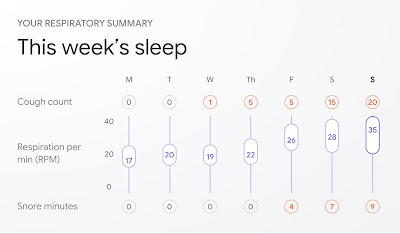
The Nest Hub displays when snoring and coughing may have disturbed a user’s sleep (top) and can track weekly trends (bottom).

To train the model, we assembled a large, hand-labeled dataset, drawing examples from the publicly available AudioSet research dataset as well as hundreds of thousands of additional real-world audio clips contributed by thousands of individuals.

Log-Mel spectrogram inputs comparing cough (left) and snore (right) audio snippets.

When a user opts in to cough and snore tracking on their bedside Nest Hub, the device first uses its Soli-based sleep algorithms to detect when a user goes to bed. Once it detects that a user has fallen asleep, it then activates its on-device sound sensing model and begins processing audio. The model works by continuously extracting spectrogram-like features from the audio input and feeding them through a convolutional neural network classifier in order to estimate the probability that coughing or snoring is happening at a given instant in time. These estimates are analyzed over the course of the night to produce a report of the overall cough count and snoring duration and highlight exactly when these events occurred.

Conclusion
The new Nest Hub, with its underlying Sleep Sensing features, is a first step in empowering users to understand their nighttime wellness using privacy-preserving radar and audio signals. We continue to research additional ways that ambient sensing and the predictive ability of consumer devices could help people better understand their daily health and wellness in a privacy-preserving way.

Acknowledgements
This work involved collaborative efforts from a multidisciplinary team of software engineers, researchers, clinicians, and cross-functional contributors. Special thanks to D. Shin for his significant contributions to this technology and blogpost, and Dr. Logan Schneider, visiting sleep neurologist affiliated with the Stanford/VA Alzheimer’s Center and Stanford Sleep Center, whose clinical expertise and contributions were invaluable to continuously guide this research. In addition to the authors, key contributors to this research from Google Health include Jeffrey Yu, Allen Jiang, Arno Charton, Jake Garrison, Navreet Gill, Sinan Hersek, Yijie Hong, Jonathan Hsu, Andi Janti, Ajay Kannan, Mukil Kesavan, Linda Lei, Kunal Okhandiar‎, Xiaojun Ping, Jo Schaeffer, Neil Smith, Siddhant Swaroop, Bhavana Koka, Anupam Pathak, Dr. Jim Taylor, and the extended team. Another special thanks to Ken Mixter for his support and contributions to the development and integration of this technology into Nest Hub. Thanks to Mark Malhotra and Shwetak Patel for their ongoing leadership, as well as the Nest, Fit, Soli, and Assistant teams we collaborated with to build and validate Sleep Sensing on Nest Hub.


1 Not intended to diagnose, cure, mitigate, prevent or treat any disease or condition. 

Categories
Misc

TextBoxGan: First GAN generating text boxes! Github repo (implemented with TF2): https://github.com/NoAchache/TextBoxGan, with all the technical and theoretical documentation, as well as a pre-trained model.

TextBoxGan: First GAN generating text boxes! Github repo (implemented with TF2): https://github.com/NoAchache/TextBoxGan, with all the technical and theoretical documentation, as well as a pre-trained model. submitted by /u/Noe_Achache
[visit reddit] [comments]
Categories
Misc

Tensorflow 2 code for Attention Mechanisms chapter of Dive into Deep Learning (D2L) book.

Tensorflow 2 code for Attention Mechanisms chapter of Dive into Deep Learning (D2L) book. submitted by /u/biswajitsahoo1111
[visit reddit] [comments]
Categories
Misc

LSTM Prediction, Coca Cola stock closing price $51.35 3/19/21

TL/DR: Teaching myself about investing and Tensorflow. My model predicts Coca Cola will close $51.35 on 3/19/2021. I have no idea what I’m doing. Do not use this to make financial decisions.

So last week I predicted Coca Cola would close at $42.56. It really closed at $50.36. I would have been better off using the lazy predictor and just assume last week’s close of $50.79 would not have moved. See my previous post:

https://www.reddit.com/r/tensorflow/comments/lzv277/silly_prediction_coca_cola_stock_closing_price/

So the first thing I did was scale my numbers. Having price points in the tens of dollars, and volume in the millions blew up my model pretty badly. My previous unscaled version had errors relative to my training data in the 10’s of dollars per week.

I scaled volume to shares outstanding, and share price to % change, and it looks like this model is performing better. The scaled model has errors much tighter. I’ve attached a histogram of my model’s error using the last 100 week’s of data. Next Friday will be the first real test though.

So the bad news. I define success as my model performing better than a “Lazy” predictor, which assumes that next week’s closing price will equal this week’s closing price. My model’s error histogram pretty much sits exactly on top of the Lazy predictor histogram.

Comparing root mean square error, my LSTM predictor is actually slightly worse…

There are a few known issues that I need to work out. I haven’t included dividend data, nor do I have a method to handle splits. I’ll need to be able to address splits if I want to include other companies.

Data is starting to get a bit messy to handle. I’m currently stuck doing some manual manipulation and manual data entry, as Alphavantage is missing historical shares outstanding. Ideally I would include float as well.

Looks like I might need to setup a SQL server locally to host all this data.

I’m starting to understand why many of the tutorials spend 80% of their time on data manipulation and only 20% on tensorflow.

submitted by /u/squirrelaway4all
[visit reddit] [comments]

Categories
Misc

MIT Researchers Use Deep Learning to Develop Real-Time 3D Holograms

Computer-generated holograms powered by deep learning could make real-time 3D holography feasible on laptops and smartphones, an advancement with potential applications in fields including virtual reality, microscopy, and 3D printing.

Computer-generated holograms powered by deep learning could make real-time 3D holography feasible on laptops and smartphones, an advancement with potential applications in fields including virtual reality, microscopy, and 3D printing.
Published this week in Nature, an MIT study outlines a novel approach called tensor holography, where researchers trained and optimized a convolutional neural network to create holograms from images with depth information. The compact network requires under 1 MB of memory, and crafts holograms within milliseconds. 

“People previously thought that with existing consumer-grade hardware, it was impossible to do real-time 3D holography computations,” said lead author Liang Shi, Ph.D. student in MIT’s Department of Electrical Engineering and Computer Science. “It’s often been said that commercially available holographic displays will be around in 10 years, yet this statement has been around for decades.”

Old-school holograms use laser beams to depict a static scene with both colors and a sense of depth. Traditionally, computer-generated holography has relied on supercomputers to simulate this optical set up, making it possible to create digital holograms that can also capture motion and be easily reproduced and shared.  

Simulating the underlying physics of a hologram, however, is computationally intensive, taking up to minutes to render a single holographic image on a clustered supercomputer.  

“Because each point in the scene has a different depth, you can’t apply the same operations for all of them,” Shi said. “That increases the complexity significantly.”

To speed things up, and increase the photorealistic precision of the holograms, the researchers turned to deep learning. 

The team created custom high-quality training data — the first such database for 3D holograms — made up of 4,000 images with depth information, and a corresponding 3D hologram for each image. Training on NVIDIA Tensor Core GPUs, the CNN learned to generate accurate holograms from images with depth information, which can be acquired by standard modern smartphones with multi-camera setups or LiDAR sensors. 

Using an NVIDIA TITAN RTX GPU and the NVIDIA TensorRT SDK for inference, the optimized neural network runs in real time, achieving a speedup of more than two orders of magnitude compared to physical simulation. The final model uses just 617 kilobytes of memory, allowing it to run interactively on low-power AI chips on mobile and edge devices. 

The resulting method not only accelerated the process, but also produced holograms with accurate occlusion and per-pixel focal control, improving the images’ realism. 

Read the news release from MIT and visit the researchers’ project page. The full paper can be found in Nature.

Categories
Offsites

LEAF: A Learnable Frontend for Audio Classification

Developing machine learning (ML) models for audio understanding has seen tremendous progress over the past several years. Leveraging the ability to learn parameters from data, the field has progressively shifted from composite, handcrafted systems to today’s deep neural classifiers that are used to recognize speech, understand music, or classify animal vocalizations such as bird calls. However, unlike computer vision models, which can learn from raw pixels, deep neural networks for audio classification are rarely trained from raw audio waveforms. Instead, they rely on pre-processed data in the form of mel filterbanks — handcrafted mel-scaled spectrograms that have been designed to replicate some aspects of the human auditory response.

Although modeling mel filterbanks for ML tasks has been historically successful, it is limited by the inherent biases of fixed features: even though using a fixed mel-scale and a logarithmic compression works well in general, we have no guarantee that they provide the best representations for the task at hand. In particular, even though matching human perception provides good inductive biases for some application domains, e.g., speech recognition or music understanding, these biases may be detrimental to domains for which imitating the human ear is not important, such as recognizing whale calls. So, in order to achieve optimal performance, the mel filterbanks should be tailored to the task of interest, a tedious process that requires an iterative effort informed by expert domain knowledge. As a consequence, standard mel filterbanks are used for most audio classification tasks in practice, even though they are suboptimal. In addition, while researchers have proposed ML systems to address these problems, such as Time-Domain Filterbanks, SincNet and Wavegram, they have yet to match the performance of traditional mel filterbanks.

In “LEAF, A Fully Learnable Frontend for Audio Classification”, accepted at ICLR 2021, we present an alternative method for crafting learnable spectrograms for audio understanding tasks. LEarnable Audio Frontend (LEAF) is a neural network that can be initialized to approximate mel filterbanks, and then be trained jointly with any audio classifier to adapt to the task at hand, while only adding a handful of parameters to the full model. We show that over a wide range of audio signals and classification tasks, including speech, music and bird songs, LEAF spectrograms improve classification performance over fixed mel filterbanks and over previously proposed learnable systems. We have implemented the code in TensorFlow 2 and released it to the community through our GitHub repository.

Mel Filterbanks: Mimicking Human Perception of Sound
The first step in the traditional approach to creating a mel filterbank is to capture the sound’s time-variability by windowing, i.e., cutting the signal into short segments with fixed duration. Then, one performs filtering, by passing the windowed segments through a bank of fixed frequency filters, that replicate the human logarithmic sensitivity to pitch. Because we are more sensitive to variations in low frequencies than high frequencies, mel filterbanks give more importance to the low-frequency range of sounds. Finally, the audio signal is compressed to mimic the ear’s logarithmic sensitivity to loudness — a sound needs to double its power for a person to perceive an increase of 3 decibels.

LEAF loosely follows this traditional approach to mel filterbank generation, but replaces each of the fixed operations (i.e., the filtering layer, windowing layer, and compression function) by a learned counterpart. The output of LEAF is a time-frequency representation (a spectrogram) similar to mel filterbanks, but fully learnable. So, for example, while a mel filterbank uses a fixed scale for pitch, LEAF learns the scale that is best suited to the task of interest. Any model that can be trained using mel filterbanks as input features, can also be trained on LEAF spectrograms.

Diagram of computation of mel filterbanks compared to LEAF spectrograms.

While LEAF can be initialized randomly, it can also be initialized in a way that approximates mel filterbanks, which have been shown to be a better starting point. Then, LEAF can be trained with any classifier to adapt to the task of interest.

Left: Mel filterbanks for a person saying “wow”. Right: LEAF’s output for the same example, after training on a dataset of speech commands.

A Parameter-Efficient Alternative to Fixed Features
A potential downside of replacing fixed features that involve no learnable parameter with a trainable system is that it can significantly increase the number of parameters to optimize. To avoid this issue, LEAF uses Gabor convolution layers that have only two parameters per filter, instead of the ~400 parameters typical of a standard convolution layer. This way, even when paired with a small classifier, such as EfficientNetB0, the LEAF model only accounts for 0.01% of the total parameters.

Top: Unconstrained convolutional filters after training for audio event classification. Bottom: LEAF filters at convergence after training for the same task.

Performance
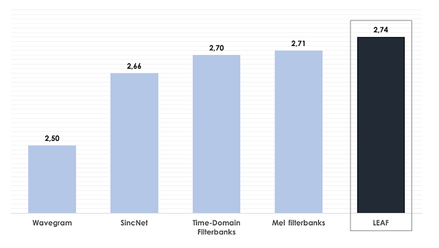
We apply LEAF to diverse audio classification tasks, including recognizing speech commands, speaker identification, acoustic scene recognition, identifying musical instruments, and finding birdsongs. On average, LEAF outperforms both mel filterbanks and previous learnable frontends, such as Time-Domain Filterbanks, SincNet and Wavegram. In particular, LEAF achieves a 76.9% average accuracy across the different tasks, compared to 73.9% for mel filterbanks. Moreover we show that LEAF can be trained in a multi-task setting, such that a single LEAF parametrization can work well across all these tasks. Finally, when combined with a large audio classifier, LEAF reaches state-of-the-art performance on the challenging AudioSet benchmark, with a 2.74 d-prime score.

D-prime score (the higher the better) of LEAF, mel filterbanks and previously proposed learnable spectrograms on the evaluation set of AudioSet.

Conclusion
The scope of audio understanding tasks keeps growing, from diagnosing dementia from speech to detecting humpback whale calls from underwater microphones. Adapting mel filterbanks to every new task can require a significant amount of hand-tuning and experimentation. In this context, LEAF provides a drop-in replacement for these fixed features, that can be trained to adapt to the task of interest, with minimal task-specific adjustments. Thus, we believe that LEAF can accelerate development of models for new audio understanding tasks.

Acknowledgements
We thank our co-authors, Olivier Teboul, Félix de Chaumont-Quitry and Marco Tagliasacchi. We also thank Dick Lyon, Vincent Lostanlen, Matt Harvey, and Alex Park for helpful discussions, and Julie Thomas for helping to design figures for this post.

Categories
Misc

Support for CUDA Unified Memory Now Available in Thrust

Thrust 1.12.0 and CUB 1.12.0 are distributed with the NVIDIA HPC SDK 21.3 and the CUDA Toolkit 11.4.

Thrust 1.12.0 is a major release providing bug fixes and performance enhancements. It includes a new thrust::universal_vector which holds data that is accessible from both host and device. This enables the use of CUDA unified memory with Thrust. Also added are new asynchronous versions of thrust::async:exclusive_scan and inclusive_scan algorithms. The synchronous versions of these have been updated to use cub::DeviceScan directly. This release deprecates support for Clang

CUB 1.12.0 is a major release providing bug fixes and performance enhancements. It includes improved Radix sort stability.  Please see the CUB 1.12 Release Notes for more information.

Both packages are available today from GitHub.  They are also distributed with the NVIDIA HPC SDK 21.3 and the CUDA Toolkit 11.4.

About Thrust and CUB

Thrust is a modern C++ parallel algorithms library which provides a std::-like interface. Thrust abstractions are agnostic of any particular parallel programming model or hardware. With Thrust, you can write code once and run it in parallel on either your CPU or GPU. CUB is a C++ library of collective primitives and utilities for parallel algorithm authors. CUB is specific to CUDA C++ and its interfaces explicitly accommodate CUDA-specific features.

Thrust and CUB are complementary and are often used together. 

Learn more: