This may seem like a basic question but I am a little confused. In this example picture I call model.evaluate. The returned message says the batch_loss is 2.1455. But I had a callback keep track of the batch loss and if I calculate the mean of the batch_loss it is 2.0925, and 2.1455 is not seen in any of the callback loss values. So… What is evaluating returning here?
If I am making a function that has two inputs, what values is `tape.gradients` expecting?
For example, if I input data in a batch size to the function `f(x,y)`, the `tape.gradient` expects both of the returned gradients to be of shape (batch size, 2), however I’m not sure what should be the contents of those Tensors. For a batch size of 3, I thought it would look something like the following:
df/dx (x_1, y_1)
df/dy (x_1, y_1)
df/dx (x_2, y_2)
df/dy (x_2, y_2)
df/dx (x_3, y_3)
df/dy (x_3, y_3)
Where the above table is a Tensor, but i have no idea what other tensor it could want for the second variable. Does anyone have an idea of what it should be? Thanks
The latest Nsight Systems 2022.1 release introduces several improvements aimed to enhance the profiling experience.
The latest update to NVIDIA Nsight Systems—a performance analysis tool designed to help developers tune and scale software across CPUs and GPUs—is now available for download. Nsight Systems 2022.1 introduces several improvements aimed to enhance the profiling experience.
Nsight Systems is part of the powerful debugging and profiling NVIDIA Nsight Tools Suite. A developer can start with Nsight Systems for an overall system view and avoid picking less efficient optimizations based on assumptions and false-positive indicators.
2022.1 highlights
Vulkan 1.3 support.
System-wide CPU backtrace sampling and CPU context switch tracing on Linux.
NVIDIA NIC metrics sampling improvements.
MPI trace improvements.
Improvements for remote profiling over SSH.
With Vulkan 1.3, you now have access to nearly two dozen new extensions. Some extensions, like VK_KHR_dynamic_rendering, help you to simplify your code while improving readability.
Other extensions, such as VK_KHR_shader_integer_dot_product or VK_EXT_pipeline_creation_cache_control, provide new functionality to help you build even better graphics applications.
This release of Nsight Systems includes support for Vulkan 1.3 that helps you solve real world problems quickly and easily.
Figure 1. Vulkan 1.3 and ray tracing leadership video
The system-wide CPU thread context switch trace and backtrace sampling feature on Linux. Users will now be able to see if other apps, OS processes and kernel might be interfering with the processes you are profiling.
Figure 2. System-wide CPU backtrace sampling and CPU context switch tracing on Linux.
Generating and labeling data to train AI models is time-consuming. Appen, helps label and annotate your data, which can then be used as inputs in the TAO Toolkit.
Building AI models from scratch requires enormous amounts of data, time, money, and expertise. This is at odds with what it takes to succeed in the AI space: fast time-to-market and the ability to quickly evolve and customize solutions. NVIDIA TAO, an AI-Model-Adaptation framework, enables you to leverage production-quality, pretrained AI models and fine-tune them in a fraction of the time compared to training from scratch.
To fine-tune these models further, or confirm the precision of your model, additional high-quality training data is required. Appen, a data annotation partner for TAO, provides access to high-quality datasets and services to label and annotate your data for your unique needs, if you don’t have the right data available.
In the post, I show you how you can use the NVIDIA TAO Toolkit, a CLI-based solution of the NVIDIA TAO framework, along with Appen’s data labeling platform to simplify the overall training process and create highly customized models for a particular use case.
After your team has identified a business problem to solve using ML, you can select from NVIDIA collection of pretrained AI models in computer vision and conversational AI. Computer vision models can include face detection models, text recognition, segmentation, and more. Then you can apply the TAO Toolkit to build, train, test, and deploy your solution.
To speed up the data collection and augmentation process, you can now use the Appen Data Annotation Platform to create the right training data for your use case. The robust platform enables you to access Appen’s global crowd of over one million skilled annotators from over 170 countries, speaking 235 languages. Appen’s data annotation platform and expertise also provide you with other resources:
High-quality datasets (for when you need data)
Human labelers sourced globally to annotate your unlabeled data
An easy-to-use platform where you can launch annotation jobs and monitor key metrics
Quality assurance checks and data security controls
With clean, high-quality data, you can adapt pretrained NVIDIA models to suit your requirements, pruning, and retraining to achieve the performance level that you need.
How to prepare your data using Appen’s platform
If you don’t already have data to use for training your model, you can either collect that data yourself or turn to Appen to source datasets that suit your use cases. The Appen Data Annotation Platform (ADAP) works with a diverse set of formats:
Audio (.wav, .mp3)
Image (.jpeg, .png)
Text (.txt)
Video (URL)
When you’re done with the data collection phase, unless you plan to work with Appen for your data collection needs, you can use Appen’s platform to quickly label the data you’ve collected. You need an Appen platform license and budget for each row of data annotation.
From there, work through the following steps to deploy a model that works specifically for your needs. For the purposes of this post, assume that you’re annotating images for an object detection model.
Prepare your data
First, load your image data into a web-accessible location: the cloud or a location that ADAP can access, such as a private Amazon S3 bucket.
Next, structure your input CSV file with two columns. The first column contains the filenames, and the second includes URLs to the images. You can provide the URLs in one of three ways:
Use publicly available URLs for your data.
Use presigned URLs.
Use Appen’s Secure Data Access tool, which you can use to attach your database securely to the platform; Appen only accesses your data when needed.
The second column contains the local file name on your device. Figure 1 shows what your CSV file may look like.
Figure 1. CSV structure for data upload in ADAP
Create your job and upload data
If you haven’t already, you can create an ADAP account and sign in. You must have an active license for the platform before running new jobs. To learn more about plans and pricing, contact Appen.
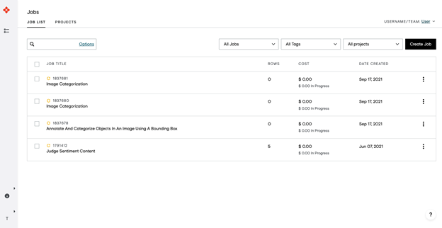
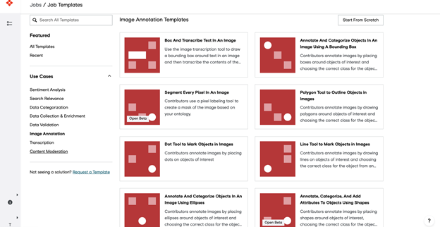
After logging in, under Jobs, choose Create a Job.
Figure 2. ADAP jobs overview page
Select the template that best fits the job (sentiment analysis, search relevance, and so on). For this example, choose Image Annotation.
Under Image Annotation, choose Annotate and Categorize Objects in an Image Using a Bounding Box. Upload your CSV file by dragging and dropping it into the Upload tab.
Design your job
Provide guidelines for Appen’s crowd of over one million data labelers on what they should be looking for and any requirements that they should be aware of. The template provides a simple job design to help you get started.
Next, choose Manage the Image Annotation Ontology, where you’ll define the classes that should be detected. Update the instructions to give more context about your use case and describe how annotators should identify and label objects in images. You can preview your job and see how an annotator will view it.
Finally, create test questions to measure and track labeler performance.
Launch job
Do a test run first before officially launching your annotation job on the platform. After you’ve launched your job, Appen’s global crowd of data labelers annotate your data to your specifications.
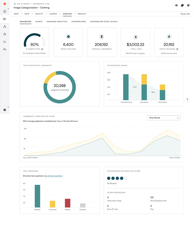
Monitor
Monitor the accuracy rate of annotations in real time. Adjust as needed in areas like job design, test questions, or annotators.
Download a report of your labeled data output by choosing Download, Full.
Convert output to KITTI format
From here, you need a script to convert your labeled data to a format that’s feedable to the TAO Toolkit, such as KITTI format.
Using the output from the previous step, you can use the following section to convert your labeled data to a format like the Pascal Visual Object Classes (VOC) format. For the full code and guide on how to convert your data, see the /Appen/public-demos GitHub repo.
Training your model
Your data annotated with Appen can now be used to train your object detection model. The TAO Toolkit allows you to train, fine-tune, prune, and export highly optimized and accurate AI models for deployment by adapting popular network architectures and backbones to your data. For this example, you can choose a YOLOV3 Object Detection model, as in the following example:
Open the internet browser on localhost and open the following URL:
http://0.0.0.0:8888
Because you are creating a YOLOv3 model, open the yolo_v3/yolo_v3.ipynb notebook. Follow the notebook instructions to train the model.
Based on results, fine-tune the model until it achieves your metric goals. If desired, you can create your own active learning loop at this stage. Prioritize data based on confidence or another selection metric using the CSV file method as described in the preceding steps. You can also load data (including inputs and predictions) beforehand so Appen’s annotators can validate the model after it’s been trained, reviewing the predictions using our domain experts and open crowd.
Pro tip: Use Workflows, an Appen Solution, to build and automate multistep data annotation projects with ease.
Iterate
Appen can further assist you with data collection and annotation in subsequent rounds of model training as you iteratively improve on your model performance. To avoid model drift or to accommodate changing business requirements, retrain your model regularly.
Conclusion
NVIDIA TAO Toolkit combined with Appen’s data platform enables you to train, fine-tune, and optimize pretrained models to get your AI solutions off the ground faster. Speed up your development times by tenfold without sacrificing quality. With the help of integrated expertise and tools from NVIDIA and Appen, you’ll be ready to launch AI with confidence.
For more information, see the following resources:
I’m looking at the MSE source documentation for help making a custom loss function, and it seems that MSE will return a single loss value no matter what, not a loss value per pair of y_true and y_pred. Could anyone help me understand this?
Learn the skills to transform raw video data from cameras into deep learning-based insights in real time
Video analytics rely on computerized processing and automatic analysis of video content to detect and determine temporal and spatial events. The field is anticipated to experience double-digit growth for the next decade, as videos are quickly becoming a primary media form for transferring information.
As the amount of video data generated grows at unprecedented rates, so does the ability and desire to analyze this information. Intelligent video analytics (IVA), which uses computer vision to extract valuable information from unstructured video data, is at the cutting edge of this emerging field.
The computer vision revolution
Computer vision, which uses deep learning models to help machines understand visual data, has improved drastically over the past few years thanks to HPC and neural networks. It transforms pixels to usable data through a range of tasks such as image classification, object detection, and segmentation.
Some of its use cases include behavior analysis, enhanced safety measures, operations management, optical inspection, and content filtering. It has also aided new industries such as autonomous vehicles, smart retail, smart cities, and smart healthcare. Recognizing the potential IVA holds, organizations are eager to develop applications that harness this technology.
Developing video AI applications
NVIDIA, through the DeepStream SDK and the TAO Toolkit, makes creating highly-performant video AI solutions easy and intuitive. The DeepStream SDK is a streaming analytics toolkit for constructing video processing pipelines. It provides the flexibility to select from various input formats, AI-based inference types, and outputs. Users also determine what to do with the results such as cold storage, composite for display, or further analysis downstream.
On the other hand, the TAO Toolkit uses transfer learning to efficiently train vision models. The software was designed with an emphasis on acceleration and optimization for video AI applications known to be computationally intensive. It can be deployed on low-power IoT devices for real-time analytics.
This course provides an easy progression of foundational understanding, important concepts, terminologies, as well as a lab portion. The hands-on walk-through of the technical components provides an opportunity to build complete video AI applications.
It’s complemented by thorough explanations in each step of the development cycle to help you confidently make implementation decisions for your own project. The course also highlights important performance considerations to optimize the video AI application and meet deployment requirements.
Upon completion, you can earn a certificate of competency and begin to develop custom applications. Intelligent video analytics is an exciting area of AI with great opportunities.
Benjamin Sokomba Dazhi, aka Benny Dee, has learned the ins and outs of the entertainment industry from many angles — first as a rapper, then as a music video director and now as a full-time animator.
The latest Nsight Graphics 2022.1 release supports Direct3D (11, 12, DXR), Vulkan 1.3, ray tracing extension, OpenGL, OpenVR, and the Oculus SDK.
Today, NVIDIA announced the latest Nsight Graphics 32022.1, which supports Direct3D (11, 12, DXR), Vulkan 1.3 ray tracing extension, OpenGL, OpenVR, and the Oculus SDK.
NVIDIA Nsight Graphics is a standalone developer tool that enables you to debug, profile, and export frames built with high-fidelity, 3D-graphic applications.
Event Details view can now link to a new Object Browser view. The Object Browser view shows objects alongside their properties, usages, and related objects.
Linux Gaming improvements.
Vertex Selection for memory analysis.
Nsight Aftermath (crash debugging) improvements.
Vulkan 1.3 support
Nsight Graphics now has day one support for Vulkan 1.3. This version includes many new extensions to support developer productivity. If you’d like to learn more about this new version of Vulkan, check out the blog post here.
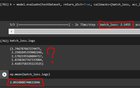
Object Browser view
The release adds the ability for you to link from the Event Details view to a new Object Browser view. The Object Browser view shows objects alongside their properties, usages, and related objects. From the Object Browser, you may also navigate to other purposed views, like resource viewers. This helps you save time by letting you quickly move from different but related viewers.
Figure 1. D3D12 events showing hyperlinks to Object Browser.
Linux gaming improvements
For Nsight Graphics users who are developing on Linux, you now have support for Ubuntu 21.04 and for Linux games, thanks to major improvements with the Linux Steam Runtime. This should make it easier to develop games that run on Linux by ensuring that the latest OS versions work correctly with Nsight Graphics.
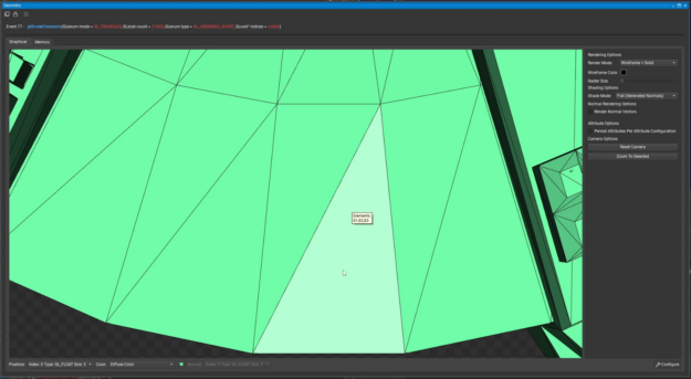
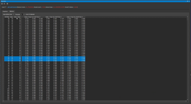
Vertex selection
With this version of Nsight Graphics, you can now select a triangle in the Graphical tab of the Geometry view and see the corresponding vertex data from the Memory tab in the Geometry view. This makes it much easier to find geometry issues as you don’t need to know the specific vertex indices before using the viewer.
Figure 2. A selected triangle (left) and the data for vertices 81, 82 and 83 (right.)
Nsight Aftermath improvements
Nsight Aftermath now shows additional information when applications crash in driver-generated shaders, like those used for ray tracing. This will assist you in narrowing down the root cause of GPU instability and allow you to provide information to NVIDIA to help fix the problem.
Many different platforms, same great performance. That’s why Vulkan is a very big deal. With the release Tuesday of Vulkan 1.3, NVIDIA continues its unparalleled record of day one driver support for this cross-platform GPU application programming interface for 3D graphics and computing. Vulkan has been created by experts from across the industry working together Read article >
The Keras Hyperband algorithm seems to work well: it simulates the various models, and when it reaches the Early Stopping condition on a model, the training of that model stops and the training of a new model starts.
What I noticed is that with this EarlyStopping callback implementation, when EarlyStopping stops the training of a model, before starting the training of the next model, the following two consecutive Python errors occur (anyway, the simulation doesn’t exit or generate exceptions, but it goes on, by simulating the successive model):
W tensorflow/core/framework/op_kernel.cc:1755] Invalid argument: ValueError: callback pyfunc_2 is not found Traceback (most recent call last): File "/home/username/anaconda3/envs/myenv/lib/python3.8/site-packages/tensorflow/python/ops/script_ops.py", line 233, in __call__ raise ValueError("callback %s is not found" % token) ValueError: callback pyfunc_2 is not found W tensorflow/core/kernels/data/generator_dataset_op.cc:103] Error occurred when finalizing GeneratorDataset iterator: Invalid argument: ValueError: callback pyfunc_2 is not found Traceback (most recent call last): File "/home/username/anaconda3/envs/myenv/lib/python3.8/site-packages/tensorflow/python/ops/script_ops.py", line 233, in __call__ raise ValueError("callback %s is not found" % token) ValueError: callback pyfunc_2 is not found [[{{node PyFunc}}]]
While if I don’t use the “min_delta” argument, these two errors don’t appear.
I also noted, looking for examples on the Internet, that, the “min_delta” argument of the EarlyStopping callback is never set – so it is always left at its default value – when tuning.
Do you know why?
PS:
I have another question:I noticed that if I set the Hyperband “max_epochs”, for example, equal to 100, the training of the model is performed by steps:
firstly, from epoch 1 to epoch 3; secondly, from 4 to 7; then, from 8 to 13; then, from 14 to 25; then, from 26 to 50; and finally, from 51 to 100.
If I set “patience=15”, I noticed that the EarlyStopping callback stops the training right after epoch 66 (thus, the first epoch at which EarlyStopping is able to operate, because 51+15=66); could it be a coincidence, or maybe should it be the normal behavior when tuning with Keras Hyperband, or what?


 The latest Nsight Systems 2022.1 release introduces several improvements aimed to enhance the profiling experience.
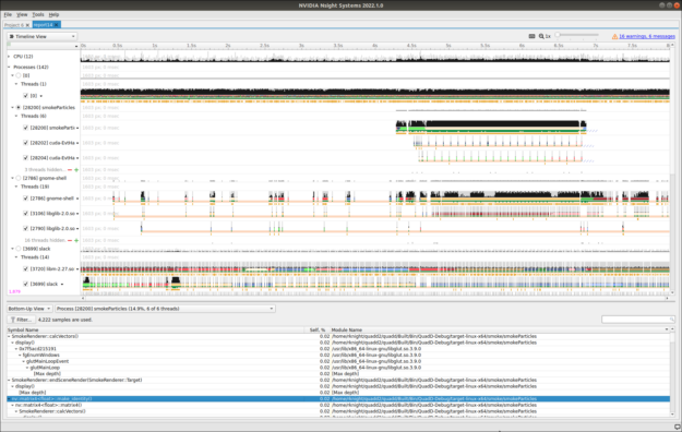
 Generating and labeling data to train AI models is time-consuming. Appen, helps label and annotate your data, which can then be used as inputs in the TAO Toolkit.
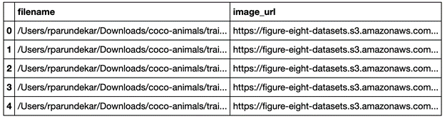
 Learn the skills to transform raw video data from cameras into deep learning-based insights in real time
 The latest Nsight Graphics 2022.1 release supports Direct3D (11, 12, DXR), Vulkan 1.3, ray tracing extension, OpenGL, OpenVR, and the Oculus SDK.
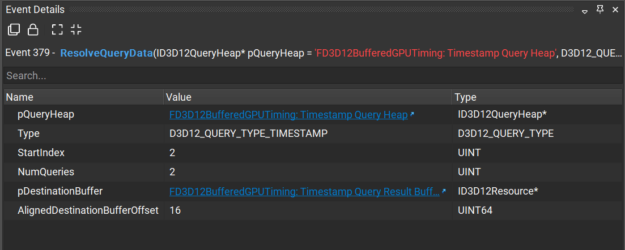