Advances in deep learning over the last few decades have been driven by a few key elements. With a small number of simple but flexible mechanisms (i.e., inductive biases such as convolutions or sequence attention), increasingly large datasets, and more specialized hardware, neural networks can now achieve impressive results on a wide range of tasks, such as image classification, machine translation, and protein folding prediction.
However, the use of large models and datasets comes at the expense of significant computational requirements. Yet, recent works suggest that large model sizes might be necessary for strong generalization and robustness, so training large models while limiting resource requirements is becoming increasingly important. One promising approach involves the use of conditional computation: rather than activating the whole network for every single input, different parts of the model are activated for different inputs. This paradigm has been featured in the Pathways vision and recent works on large language models, while it has not been well explored in the context of computer vision.
In “Scaling Vision with Sparse Mixture of Experts”, we present V-MoE, a new vision architecture based on a sparse mixture of experts, which we then use to train the largest vision model to date. We transfer V-MoE to ImageNet and demonstrate matching state-of-the-art accuracy while using about 50% fewer resources than models of comparable performance. We have also open-sourced the code to train sparse models and provided several pre-trained models.
Vision Mixture of Experts (V-MoEs)
Vision Transformers (ViT) have emerged as one of the best architectures for vision tasks. ViT first partitions an image into equally-sized square patches. These are called tokens, a term inherited from language models. Still, compared to the largest language models, ViT models are several orders of magnitude smaller in terms of number of parameters and compute.
To massively scale vision models, we replace some dense feedforward layers (FFN) in the ViT architecture with a sparse mixture of independent FFNs (which we call experts). A learnable router layer selects which experts are chosen (and how they are weighted) for every individual token. That is, different tokens from the same image may be routed to different experts. Each token is only routed to at most K (typically 1 or 2) experts, among a total of E experts (in our experiments, E is typically 32). This allows scaling the model’s size while keeping its computation per token roughly constant. The figure below shows the structure of the encoder blocks in more detail.
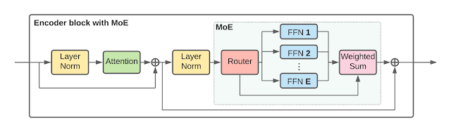 |
| V-MoE Transformer Encoder block. |
Experimental Results
We first pre-train the model once on JFT-300M, a large dataset of images. The left plot below shows our pre-training results for models of all sizes: from the small S/32 to the huge H/14.
We then transfer the model to new downstream tasks (such as ImageNet), by using a new head (the last layer in a model). We explore two transfer setups: either fine-tuning the entire model on all available examples of the new task, or freezing the pre-trained network and tuning only the new head using a few examples (known as few-shot transfer). The right plot in the figure below summarizes our transfer results to ImageNet, training on only 5 images per class (called 5-shot transfer).
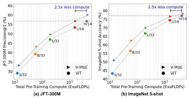 |
| JFT-300M Precision@1 and ImageNet 5-shot accuracy. Colors represent different ViT variants and markers represent either standard ViT (●), or V-MoEs (▸) with expert layers on the last n even blocks. We set n=2 for all models, except V-MoE-H where n=5. Higher indicates better performance, with more efficient models being to the left. |
In both cases, the sparse model strongly outperforms its dense counterpart at a given amount of training compute (shown by the V-MoE line being above the ViT line), or achieves similar performance much faster (shown by the V-MoE line being to the left of the ViT line).
To explore the limits of vision models, we trained a 15-billion parameter model with 24 MoE layers (out of 48 blocks) on an extended version of JFT-300M. This massive model — the largest to date in vision as far as we know — achieved 90.35% test accuracy on ImageNet after fine-tuning, near the current state-of-the-art.
Priority Routing
In practice, due to hardware constraints, it is not efficient to use buffers with a dynamic size, so models typically use a pre-defined buffer capacity for each expert. Assigned tokens beyond this capacity are dropped and not processed once the expert becomes “full”. As a consequence, higher capacities yield higher accuracy, but they are also more computationally expensive.
We leverage this implementation constraint to make V-MoEs faster at inference time. By decreasing the total combined buffer capacity below the number of tokens to be processed, the network is forced to skip processing some tokens in the expert layers. Instead of choosing the tokens to skip in some arbitrary fashion (as previous works did), the model learns to sort tokens according to an importance score. This maintains high quality predictions while saving a lot of compute. We refer to this approach as Batch Priority Routing (BPR), illustrated below.
 |
| Under high capacity, both vanilla and priority routing work well as all patches are processed. However, when the buffer size is reduced to save compute, vanilla routing selects arbitrary patches to process, often leading to poor predictions. BPR smartly prioritizes important patches resulting in better predictions at lower computational costs. |
Dropping the right tokens turns out to be essential to deliver high-quality and more efficient inference predictions. When the expert capacity decreases, performance quickly decreases with the vanilla routing mechanism. Conversely, BPR is much more robust to low capacities.
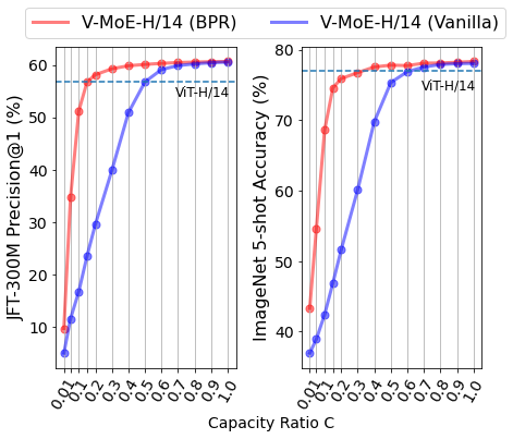 |
| Performance versus inference capacity buffer size (or ratio) C for a V-MoE-H/14 model with K=2. Even for large C’s, BPR improves performance; at low C the difference is quite significant. BPR is competitive with dense models (ViT-H/14) by processing only 15-30% of the tokens. |
Overall, we observed that V-MoEs are highly flexible at inference time: for instance, one can decrease the number of selected experts per token to save time and compute, without any further training on the model weights.
Exploring V-MoEs
Because much is yet to be discovered about the internal workings of sparse networks, we also explored the routing patterns of the V-MoE.
One hypothesis is that routers would learn to discriminate and assign tokens to experts based on some semantic grounds (the “car” expert, the “animal” experts, and so on). To test this, below we show plots for two different MoE layers (a very early-on one, and another closer to the head). The x-axis corresponds to each of the 32 experts, and the y-axis shows the ID of the image classes (from 1 to 1000). Each entry in the plot shows how often an expert was selected for tokens corresponding to the specific image class, with darker colors indicating higher frequency. While in the early layers there is little correlation, later in the network, each expert receives and processes tokens from only a handful of classes. Therefore, we can conclude that some semantic clustering of the patches emerges in the deeper layers of the network.
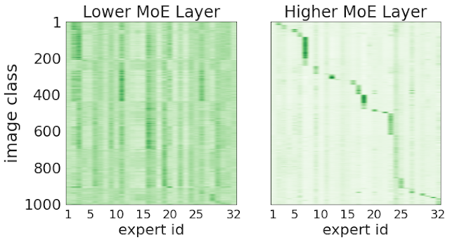 |
| Higher routing decisions correlate with image classes. We show two MoE layers of a V-MoE-H/14. The x-axis corresponds to the 32 experts in a layer. The y-axis are the 1000 ImageNet classes; orderings for both axes are different across plots (to highlight correlations). For each pair (expert e, class c) we show the average routing weight for the tokens corresponding to all images with class c for that particular expert e. |
Final Thoughts
We train very large vision models using conditional computation, delivering significant improvements in representation and transfer learning for relatively little training cost. Alongside V-MoE, we introduced BPR, which requires the model to process only the most useful tokens in the expert layers.
We believe this is just the beginning of conditional computation at scale for computer vision; extensions include multi-modal and multi-task models, scaling up the expert count, and improving transfer of the representations produced by sparse models. Heterogeneous expert architectures and conditional variable-length routes are also promising directions. Sparse models can especially help in data rich domains such as large-scale video modeling. We hope our open-source code and models help attract and engage researchers new to this field.
Acknowledgments
We thank our co-authors: Basil Mustafa, Maxim Neumann, Rodolphe Jenatton, André Susano Pinto, Daniel Keysers, and Neil Houlsby. We thank Alex Kolesnikov, Lucas Beyer, and Xiaohua Zhai for providing continuous help and details about scaling ViT models. We are also grateful to Josip Djolonga, Ilya Tolstikhin, Liam Fedus, and Barret Zoph for feedback on the paper; James Bradbury, Roy Frostig, Blake Hechtman, Dmitry Lepikhin, Anselm Levskaya, and Parker Schuh for invaluable support helping us run our JAX models efficiently on TPUs; and many others from the Brain team for their support. Finally, we would also like to thank and acknowledge Tom Small for the awesome animated figure used in this post.

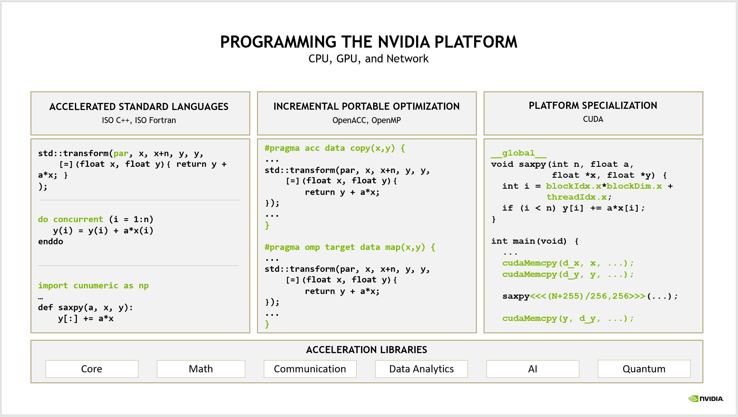
 Learn how standard language parallelism can be used for programming accelerated computing applications on NVIDIA GPUs with ISO C++, ISO Fortran, or Python.