Posted by Jaqui Herman and Cat Armato, Program Managers
This week marks the beginning of the 35th annual Conference on Neural Information Processing Systems (NeurIPS 2021), the biggest machine learning conference of the year. NeurIPS 2021 will be held virtually and includes invited talks, demonstrations and presentations of some of the latest in machine learning research. This year, NeurIPS also announced a new Datasets and Benchmarks track, which will include publications, talks, posters, and discussions related to this research area.
Google will have a strong presence with more than 170 accepted papers, additionally contributing to and learning from the broader academic research community via talks, posters, workshops, and tutorials. You can learn more about our work being presented in the list below (Google affiliations highlighted in bold).
Organizing Committee
Communications Co-Chair: Emily Denton
Program Co-Chair: Yann Dauphin
Workshop Co-Chair: Sanmi Koyejo
Senior Area Chairs: Alekh Agarwal, Amir Globerson, Been Kim, Charles Sutton, Claudio Gentile, Corinna Cortes, Dale Schuurmans, David Duvenaud, Elad Hazan, Hugo Larochelle, Jean-Philippe Vert, Kevin Murphy, Marco Cuturi, Mehryar Mohri, Mohammad Ghavamzadeh, Samory Kpotufe, Sanjiv Kumar, Satyen Kale, Sergey Levine, Tara N. Sainath, Yishay Mansour
Area Chairs: Abhishek Kumar, Abhradeep Guha Thakurta, Alex Kulesza, Alexander A. Alemi, Alexander T. Toshev, Amin Karbasi, Amit Daniely, Ananda Theertha Suresh, Ankit Singh Rawat, Ashok Cutkosky, Badih Ghazi, Balaji Lakshminarayanan, Ben Poole, Bo Dai, Boqing Gong, Chelsea Finn, Chiyuan Zhang, Christian Szegedy, Cordelia Schmid, Craig Boutilier, Cyrus Rashtchian, D. Sculley, Daniel Keysers, David Ha, Denny Zhou, Dilip Krishnan, Dumitru Erhan, Dustin Tran, Ekin Dogus Cubuk, Fabian Pedregosa, George Tucker, Hanie Sedghi, Hanjun Dai, Heinrich Jiang, Hossein Mobahi, Izhak Shafran, Jaehoon Lee, Jascha Sohl-Dickstein, Jasper Snoek, Jeffrey Pennington, Jelani Nelson, Jieming Mao, Justin Gilmer, Karol Hausman, Karthik Sridharan, Kevin Swersky, Maithra Raghu, Mario Lucic, Mathieu Blondel, Matt Kusner, Matthew Johnson, Matthieu Geist, Ming-Hsuan Yang, Mohammad Mahdian, Mohammad Norouzi, Nal Kalchbrenner, Naman Agarwal, Nicholas Carlini, Nicolas Papernot, Olivier Bachem, Olivier Pietquin, Paul Duetting, Praneeth Netrapalli, Pranjal Awasthi, Prateek Jain, Quentin Berthet, Renato Paes Leme, Richard Nock, Rif A. Saurous, Rose Yu, Roy Frostig, Samuel Stern Schoenholz, Sashank J. Reddi, Sercan O. Arik, Sergei Vassilvitskii, Sergey Ioffe, Shay Moran, Silvio Lattanzi, Simon Kornblith, Srinadh Bhojanapalli, Thang Luong, Thomas Steinke, Tim Salimans, Tomas Pfister, Tomer Koren, Uri Stemmer, Vahab Mirrokni, Vikas Sindhwani, Vincent Dumoulin, Virginia Smith, Vladimir Braverman, W. Ronny Huang, Wen Sun, Yang Li, Yasin Abbasi-Yadkori, Yinlam Chow,Yujia Li, Yunhe Wang, Zoltán Szabó
NeurIPS Foundation Board 2021: Michael Mozer, Corinna Cortes, Hugo Larochelle, John C. Platt, Fernando Pereira
Test of Time Award
Online Learning for Latent Dirichlet Allocation
Matthew D. Hoffman†, David M. Blei, Francis Bach
Publications
Deep Reinforcement Learning at the Edge of the Statistical Precipice (see blog post)
Outstanding Paper Award Recipient
Rishabh Agarwal, Max Schwarzer, Pablo Samuel Castro, Aaron Courville, Marc G. Bellemare
A Separation Result Between Data-Oblivious and Data-Aware Poisoning Attacks
Samuel Deng, Sanjam Garg, Somesh Jha, Saeed Mahloujifar, Mohammad Mahmoody, Abhradeep Guha Thakurta
Adversarial Robustness of Streaming Algorithms Through Importance Sampling
Vladimir Braverman, Avinatan Hassidim, Yossi Matias, Mariano Schain, Sandeep Silwal, Samson Zhou
Aligning Silhouette Topology for Self-Adaptive 3D Human Pose Recovery
Mugallodi Rakesh, Jogendra Nath Kundu, Varun Jampani, R. Venkatesh Babu
Attention Bottlenecks for Multimodal Fusion
Arsha Nagrani, Shan Yang, Anurag Arnab, Aren Jansen, Cordelia Schmid, Chen Sun
Autonomous Reinforcement Learning via Subgoal Curricula
Archit Sharma, Abhishek Gupta, Sergey Levine, Karol Hausman, Chelsea Finn
Calibration and Consistency of Adversarial Surrogate Losses
Pranjal Awasthi, Natalie S. Frank, Anqi Mao, Mehryar Mohri, Yutao Zhong
Compressive Visual Representations
Kuang-Huei Lee, Anurag Arnab, Sergio Guadarrama, John Canny, Ian Fischer
Counterfactual Invariance to Spurious Correlations in Text Classification
Victor Veitch, Alexander D’Amour, Steve Yadlowsky, Jacob Eisenstein
Deep Learning Through the Lens of Example Difficulty
Robert J.N. Baldock, Hartmut Maennel, Behnam Neyshabur
Deep Neural Networks as Point Estimates for Deep Gaussian Processes
Vinent Dutordoir, James Hensman, Mark van der Wilk, Carl Henrik Ek, Zoubin Ghahramani, Nicolas Durrande
Delayed Gradient Averaging: Tolerate the Communication Latency for Federated Learning
Ligeng Zhu, Hongzhou Lin, Yao Lu, Yujun Lin, Song Han
Discrete-Valued Neural Communication
Dianbo Liu, Alex Lamb, Kenji Kawaguchi, Anirudh Goyal, Chen Sun, Michael Curtis Mozer, Yoshua Bengio
Do Vision Transformers See Like Convolutional Neural Networks?
Maithra Raghu, Thomas Unterthiner, Simon Kornblith, Chiyuan Zhang, Alexey Dosovitskiy
Dueling Bandits with Team Comparisons
Lee Cohen, Ulrike Schmidt-Kraepelin, Yishay Mansour
End-to-End Multi-Modal Video Temporal Grounding
Yi-Wen Chen, Yi-Hsuan Tsai, Ming-Hsuan Yang
Environment Generation for Zero-Shot Compositional Reinforcement Learning
Izzeddin Gur, Natasha Jaques, Yingjie Miao, Jongwook Choi, Manoj Tiwari, Honglak Lee, Aleksandra Faust
H-NeRF: Neural Radiance Fields for Rendering and Temporal Reconstruction of Humans in Motion
Hongyi Xu, Thiemo Alldieck, Cristian Sminchisescu
Improving Calibration Through the Relationship with Adversarial Robustness
Yao Qin, Xuezhl Wang, Alex Beutel, Ed Chi
Learning Generalized Gumbel-Max Causal Mechanisms
Guy Lorberbom, Daniel D. Johnson, Chris J. Maddison, Daniel Tarlow, Tamir Hazan
MICo: Improved Representations via Sampling-Based State Similarity for Markov Decision Processes
Pablo Samuel Castro, Tyler Kastner, Prakash Panangaden, Mark Rowland
Near-Optimal Lower Bounds For Convex Optimization For All Orders of Smoothness
Ankit Garg, Robin Kothari, Praneeth Netrapalli, Suhail Sherif
Neural Circuit Synthesis from Specification Patterns
Frederik Schmitt, Christopher Hahn, Markus N. Rabe, Bernd Finkbeiner
Non-Local Latent Relation Distillation for Self-Adaptive 3D Human Pose Estimation
Jogendra Nath Kundu, Siddharth Seth, Anirudh Jamkhandi, Pradyumna YM, Varun Jampani, Anirban Chakraborty, R. Venkatesh Babu
Object-Aware Contrastive Learning for Debiased Scene Representation
Sangwoo Mo, Hyunwoo Kang, Kihyuk Soh, Chun-Liang Li, Jinwoo Shin
On Density Estimation with Diffusion Models
Diederik P. Kingma, Tim Salimans, Ben Poole, Jonathan Ho
On Margin-Based Cluster Recovery with Oracle Queries
Marco Bressan, Nicolo Cesa-Bianchi, Silvio Lattanzi, Andrea Paudice
On Model Calibration for Long-Tailed Object Detection and Instance Segmentation
Tai-Yu Pan, Cheng Zhang, Yandong Li, Hexiang Hu, Dong Xuan, Soravit Changpinyo, Boqing Gong, Wei-Lun Chao
Parallelizing Thompson Sampling
Amin Karbasi, Vahab Mirrokni, Mohammad Shadravan
Reverse-Complement Equivariant Networks for DNA Sequences
Vincent Mallet, Jean-Philippe Vert
Revisiting ResNets: Improved Training and Scaling Strategies
Irwan Bello, William Fedus, Xianzhi Du, Ekin Dogus Cubuk, Aravind Srinivas, Tsung-Yi Lin, Jonathon Shlens, Barret Zoph
Revisiting the Calibration of Modern Neural Networks
Matthias Minderer, Josip Djolonga, Rob Romijnders, Frances Ann Hubis, Xiaohua Zhai, Neil Houlsby, Dustin Tran, Mario Lucic
Scaling Vision with Sparse Mixture of Experts
Carlos Riquelme, Joan Puigcerver, Basil Mustafa, Maxim Neumann, Rodolphe Jenatton, André Susano Pinto, Daniel Keysers, Neil Houlsby
SE(3)-Equivariant Prediction of Molecular Wavefunctions and Electronic Densities
Oliver Thorsten Unke, Mihail Bogojeski, Michael Gastegger, Mario Geiger, Tess Smidt, Klaus Robert Muller
Stateful ODE-Nets Using Basis Function Expansions
Alejandro Francisco Queiruga, N. Benjamin Erichson, Liam Hodgkinson, Michael W. Mahoney
Statistically and Computationally Efficient Linear Meta-Representation Learning
Kiran Koshy Thekumparampil, Prateek Jain, Praneeth Netrapalli, Sewoong Oh
Streaming Belief Propagation for Community Detection
Yuchen Wu, Jakab Tardos, Mohammad Hossein Bateni, André Linhares, Filipe Miguel Gonçalves de Almeida, Andrea Montanari, Ashkan Norouzi-Fard
Synthetic Design: An Optimization Approach to Experimental Design with Synthetic Controls
Nick Doudchenko, Khashayar Khosravi, Jean Pouget-Abadie, Sebastien Lahaie, Miles Lubin, Vahab Mirrokni, Jann Spiess, Guido Imbens
The Difficulty of Passive Learning in Deep Reinforcement Learning
George Ostrovski, Pablo Samuel Castro, Will Dabney
The Pareto Frontier of Model Selection for General Contextual Bandits
Teodor Marinov, Julian Zimmert
VATT: Transformers for Multimodal Self-Supervised Learning from Raw Video, Audio and Text
Hassan Akbari, Liangzhe Yuan, Rui Qian, Wei-Hong Chuang, Shih-Fu Chang, Yin Cui, Boqing Gong
Co-Adaptation of Algorithmic and Implementational Innovations in Inference-Based Deep Reinforcement Learning
Hiroki Furuta, Tadashi Kozuno, Tatsuya Matsushima, Yutaka Matsuo, Shixiang Gu
Conservative Data Sharing for Multi-Task Offline Reinforcement Learning
Tianhe Yu, Aviral Kumar, Yevgen Chebotar, Karol Hausman, Sergey Levine, Chelsea Finn
Does Knowledge Distillation Really Work?
Samuel Stanton, Pavel Izmailov, Polina Kirichenko, Alexander A. Alemi, Andrew Gordon Wilson
Exponential Graph is Provably Efficient for Decentralized Deep Training
Bicheng Ying, Kun Yuan, Yiming Chen, Hanbin Hu, Pan Pan, Wotao Yin
Faster Matchings via Learned Duals
Michael Dinitz, Sungjin Im, Thomas Lavastida, Benjamin Moseley, Sergei Vassilvitskii
Improved Transformer for High-Resolution GANs
Long Zhao, Zizhao Zhang, Ting Chen, Dimitris N. Metaxas, Han Zhang
Near-Optimal Offline and Streaming Algorithms for Learning Non-Linear Dynamical Systems
Prateek Jain, Suhas S. Kowshik, Dheeraj Mysore Nagaraj, Praneeth Netrapalli
Nearly Horizon-Free Offline Reinforcement Learning
Tongzheng Ren, Jialian Li, Bo Dai, Simon S. Du, Sujay Sanghavi
Overparameterization Improves Robustness to Covariate Shift in High Dimensions
Nilesh Tripuraneni, Ben Adlam, Jeffrey Pennington
Pay Attention to MLPs
Hanxiao Liu, Zihang Dai, David R. So, Quoc V. Le
PLUR: A Unifying, Graph-Based View of Program Learning, Understanding, and Repair
Zimin Chen*, Vincent Josua Hellendoorn*, Pascal Lamblin, Petros Maniatis, Pierre-Antoine Manzagol, Daniel Tarlow, Subhodeep Moitra
Prior-Independent Dynamic Auctions for a Value-Maximizing Buyer
Yuan Deng, Hanrui Zhang
Remember What You Want to Forget: Algorithms for Machine Unlearning
Ayush Sekhari, Jayadev Acharya, Gautam Kamath, Ananda Theertha Suresh
Reverse Engineering Learned Optimizers Reveals Known and Novel Mechanisms
Niru Maheswaranathan*, David Sussillo*, Luke Metz, Ruoxi Sun, Jascha Sohl-Dickstein
Revisiting 3D Object Detection From an Egocentric Perspective
Boyang Deng, Charles R. Qi, Mahyar Najibi, Thomas Funkhouser, Yin Zhou, Dragomir Anguelov
Robust Auction Design in the Auto-Bidding World
Santiago Balseiro, Yuan Deng, Jieming Mao, Vahab Mirrokni, Song Zuo
Shift-Robust GNNs: Overcoming the Limitations of Localized Graph Training Data
Qi Zhu, Natalia Ponomareva, Jiawei Han, Bryan Perozzi
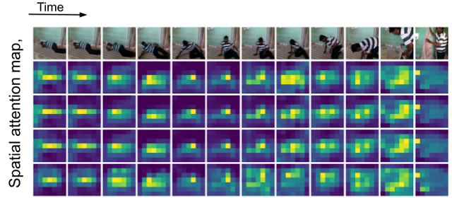
Understanding How Encoder-Decoder Architectures Attend
Kyle Aitken, Vinay V. Ramasesh, Yuan Cao, Niru Maheswaranathan
Understanding the Effect of Stochasticity in Policy Optimization
Jincheng Mei, Bo Dai, Chenjun Xiao, Csaba Szepesvari, Dale Schuurmans
Accurately Solving Rod Dynamics with Graph Learning
Han Shao, Tassilo Kugelstadt, Torsten Hädrich, Wojtek Palubicki, Jan Bender, Sören Pirk, Dominik L. Michels
GradInit: Learning to Initialize Neural Networks for Stable and Efficient Training
Chen Zhu, Renkun Ni, Zheng Xu, Kezhi Kong, W. Ronny Huang, Tom Goldstein
Learnability of Linear Thresholds from Label Proportions
Rishi Saket
MLP-Mixer: An All-MLP Architecture for Vision
Ilya Tolstikhin, Neil Houlsby, Alexander Kolesnikov, Lucas Beyer, Xiaohua Zhai, Thomas Unterthiner, Jessica Yung, Andreas Steiner, Daniel Keysers, Jakob Uszkoreit, Mario Lucic, Alexey Dosovitskiy
Neural Additive Models: Interpretable Machine Learning with Neural Nets
Rishabh Agarwal, Levi Melnick, Nicholas Frosst, Xuezhou Zhang, Ben Lengerich, Rich Caruana, Geoffrey Hinton
Neural Production Systems
Anirudh Goyal, Aniket Didolkar, Nan Rosemary Ke, Charles Blundell, Philippe Beaudoin, Nicolas Heess, Michael Mozer, Yoshua Bengio
Physics-Aware Downsampling with Deep Learning for Scalable Flood Modeling
Niv Giladi, Zvika Ben-Haim, Sella Nevo, Yossi Matias, Daniel Soudry
Shape from Blur: Recovering Textured 3D Shape and Motion of Fast Moving Objects
Denys Rozumnyi, Martin R. Oswald, Vittorio Ferrari, Marc Pollefeys
What Matters for Adversarial Imitation Learning?
Manu Orsini, Anton Raichuk, Léonard Hussenot, Damien Vincent, Robert Dadashi, Sertan Girgin, Matthieu Geist, Olivier Bachem, Olivier Pietquin, Marcin Andrychowicz
A Convergence Analysis of Gradient Descent on Graph Neural Networks
Pranjal Awasthi, Abhimanyu Das, Sreenivas Gollapudi
A Geometric Analysis of Neural Collapse with Unconstrained Features
Zhihui Zhu, Tianyu Ding, Jinxin Zhou, Xiao Li, Chong You, Jeremias Sulam, Qing Qu
Agnostic Reinforcement Learning with Low-Rank MDPs and Rich Observations
Christoph Dann, Yishay Mansour, Mehryar Mohri, Ayush Sekhari, Karthik Sridharan
Controlled Text Generation as Continuous Optimization with Multiple Constraints
Sachin Kumar, Eric Malmi, Aliaksei Severyn, Yulia Tsvetkov
Coupled Gradient Estimators for Discrete Latent Variables
Zhe Dong, Andriy Mnih, George Tucker
Detecting Errors and Estimating Accuracy on Unlabeled Data with Self-Training Ensembles
Jiefeng Chen*, Frederick Liu, Besim Avci, Xi Wu, Yingyu Liang, Somesh Jha
Neural Active Learning with Performance Guarantees
Zhilei Wang, Pranjal Awasthi, Christoph Dann, Ayush Sekhari, Claudio Gentile
Optimal Sketching for Trace Estimation
Shuli Jiang, Hai Pham, David Woodruff, Qiuyi (Richard) Zhang
Representing Long-Range Context for Graph Neural Networks with Global Attention
Zhanghao Wu, Paras Jain, Matthew A. Wright, Azalia Mirhoseini, Joseph E. Gonzalez, Ion Stoica
Scaling Up Exact Neural Network Compression by ReLU Stability
Thiago Serra, Xin Yu, Abhinav Kumar, Srikumar Ramalingam
Soft Calibration Objectives for Neural Networks
Archit Karandikar, Nicholas Cain, Dustin Tran, Balaji Lakshminarayanan, Jonathon Shlens, Michael Curtis Mozer, Rebecca Roelofs
Sub-Linear Memory: How to Make Performers SLiM
Valerii Likhosherstov, Krzysztof Choromanski, Jared Davis, Xingyou Song, Adrian Weller
A New Theoretical Framework for Fast and Accurate Online Decision-Making
Nicolò Cesa-Bianchi, Tommaso Cesari, Yishay Mansour, Vianney Perchet
Bridging the Gap Between Practice and PAC-Bayes Theory in Few-Shot Meta-Learning
Nan Ding, Xi Chen, Tomer Levinboim, Sebastian Goodman, Radu Soricut
Differentially Private Multi-Armed Bandits in the Shuffle Model
Jay Tenenbaum, Haim Kaplan, Yishay Mansour, Uri Stemmer
Efficient and Local Parallel Random Walks
Michael Kapralov, Silvio Lattanzi, Navid Nouri, Jakab Tardos
Improving Anytime Prediction with Parallel Cascaded Networks and a Temporal-Difference Loss
Michael Louis Iuzzolino, Michael Curtis Mozer, Samy Bengio*
It Has Potential: Gradient-Driven Denoisers for Convergent Solutions to Inverse Problems
Regev Cohen, Yochai Blau, Daniel Freedman, Ehud Rivlin
Learning to Combine Per-Example Solutions for Neural Program Synthesis
Disha Shrivastava, Hugo Larochelle, Daniel Tarlow
LLC: Accurate, Multi-purpose Learnt Low-Dimensional Binary Codes
Aditya Kusupati, Matthew Wallingford, Vivek Ramanujan, Raghav Somani, Jae Sung Park, Krishna Pillutla, Prateek Jain, Sham Kakade, Ali Farhadi
There Is No Turning Back: A Self-Supervised Approach for Reversibility-Aware Reinforcement Learning (see blog post)
Nathan Grinsztajn, Johan Ferret, Olivier Pietquin, Philippe Preux, Matthieu Geist
A Near-Optimal Algorithm for Debiasing Trained Machine Learning Models
Ibrahim Alabdulmohsin, Mario Lucic
Adaptive Sampling for Minimax Fair Classification
Shubhanshu Shekhar, Greg Fields, Mohammad Ghavamzadeh, Tara Javidi
Asynchronous Stochastic Optimization Robust to Arbitrary Delays
Alon Cohen, Amit Daniely, Yoel Drori, Tomer Koren, Mariano Schain
Boosting with Multiple Sources
Corinna Cortes, Mehryar Mohri, Dmitry Storcheus, Ananda Theertha Suresh
Breaking the Centralized Barrier for Cross-Device Federated Learning
Sai Praneeth Karimireddy, Martin Jaggi, Satyen Kale, Mehryar Mohri, Sashank J. Reddi, Sebastian U. Stitch, Ananda Theertha Sureshi
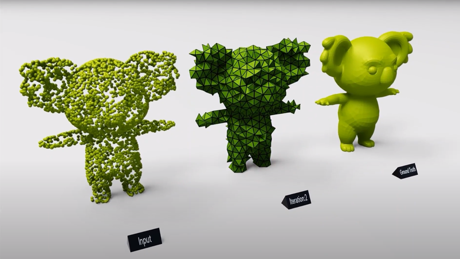
Canonical Capsules: Self-Supervised Capsules in Canonical Pose
Weiwei Sun, Andrea Tagliasacchi, Boyang Deng, Sara Sabour, Soroosh Yazdani, Geoffrey Hinton, Kwang Moo Yi
Contextual Recommendations and Low-Regret Cutting-Plane Algorithms
Sreenivas Gollapudi, Guru Guruganesh, Kostas Kollias, Pasi Manurangsi, Renato Paes Leme, Jon Schneider
Decision Transformer: Reinforcement Learning via Sequence Modeling
Lili Chen, Kevin Lu, Aravind Rajeswaran, Kimin Lee|Aditya Grover, Michael Laskin, Pieter Abbeel, Aravind Srinivas, Igor Mordatch
Deep Learning on a Data Diet: Finding Important Examples Early in Training
Mansheej Paul, Surya Ganguli, Gintare Karolina Dziugaite
Deep Learning with Label Differential Privacy
Badih Ghazi, Noah Golowich*, Ravi Kumar, Pasin Manurangsi, Chiyuan Zhang
Efficient Training of Retrieval Models Using Negative Cache
Erik Lindgren, Sashank J. Reddi, Ruiqi Guo, Sanjiv Kumar
Exploring Cross-Video and Cross-Modality Signals for Weakly-Supervised Audio-Visual Video Parsing
Yan-Bo Lin, Hung-Yu Tseng, Hsin-Ying Lee, Yen-Yu Lin, Ming-Hsuan Yang
Federated Reconstruction: Partially Local Federated Learning
Karan Singhal, Hakim Sidahmed, Zachary Garrett, Shanshan Wu, Keith Rush, Sushant Prakash
Framing RNN as a Kernel Method: A Neural ODE Approach
Adeline Fermanian, Pierre Marion, Jean-Philippe Vert, Gérard Biau
Learning Semantic Representations to Verify Hardware Designs
Shobha Vasudevan, Wenjie Jiang, David Bieber, Rishabh Singh, Hamid Shojaei, C. Richard Ho, Charles Sutton
Learning with User-Level Privacy
Daniel Asher Nathan Levy*, Ziteng Sun*, Kareem Amin, Satyen Kale, Alex Kulesza, Mehryar Mohri, Ananda Theertha Suresh
Logarithmic Regret from Sublinear Hints
Aditya Bhaskara, Ashok Cutkosky, Ravi Kumar, Manish Purohit
Margin-Independent Online Multiclass Learning via Convex Geometry
Guru Guruganesh, Allen Liu, Jon Schneider, Joshua Ruizhi Wang
Multiclass Boosting and the Cost of Weak Learning
Nataly Brukhim, Elad Hazan, Shay Moran, Indraneel Mukherjee, Robert E. Schapire
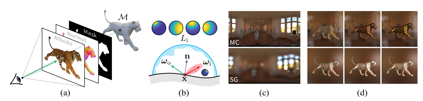
Neural-PIL: Neural Pre-integrated Lighting for Reflectance Decomposition
Mark Boss, Varun Jampani, Raphael Braun, Ce Liu*, Jonathan T. Barron, Hendrik Lensch
Never Go Full Batch (in Stochastic Convex Optimization)
Idan Amir, Yair Carmon, Tomer Koren, Roi Livni
On Large-Cohort Training for Federated Learning
Zachary Charles, Zachary Garrett, Zhouyuan Huo, Sergei Shmulyian, Virginia Smith
On the Sample Complexity of Privately Learning Axis-Aligned Rectangles
Menachem Sadigurschi, Uri Stemmer
Online Control of Unknown Time-Varying Dynamical Systems
Edgar Minasyan, Paula Gradu, Max Simchowitz, Elad Hazan
Online Knapsack with Frequency Predictions
Sungjin Im, Ravi Kumar,Mahshid Montazer Qaem, Manish Purohit
Optimal Rates for Random Order Online Optimization
Uri Sherman, Tomer Koren, Yishay Mansour
Oracle-Efficient Regret Minimization in Factored MDPs with Unknown Structure
Aviv Rosenberg, Yishay Mansour
Practical Large-Scale Linear Programming Using Primal-Dual Hybrid Gradient
David Applegate, Mateo Díaz*, Oliver Hinder, Haihao Lu*, Miles Lubin, Brendan O’Donoghue, Warren Schudy
Private and Non-Private Uniformity Testing for Ranking Data
Robert Istvan Busa-Fekete, Dimitris Fotakis, Manolis Zampetakis
Privately Learning Subspaces
Vikrant Singhal, Thomas Steinke
Provable Representation Learning for Imitation with Contrastive Fourier Features
Ofir Nachum, Mengjiao Yang
Safe Reinforcement Learning with Natural Language Constraints
Tsung-Yen Yang, Michael Hu, Yinlam Chow, Peter J. Ramadge, Karthik Narasimhan
Searching for Efficient Transformers for Language Modeling
David R. So, Wojciech Mańke, Hanxiao Liu, Zihang Dai, Noam Shazeer, Quoc V. Le
SLOE: A Faster Method for Statistical Inference in High-Dimensional Logistic Regression
Steve Yadlowsky, Taedong Yun, Cory McLean, Alexander D’Amour
Streaming Linear System Identification with Reverse Experience Replay
Prateek Jain, Suhas S. Kowshik, Dheeraj Mysore Nagaraj, Praneeth Netrapalli
The Skellam Mechanism for Differentially Private Federated Learning
Naman Agarwal, Peter Kairouz, Ziyu Liu*
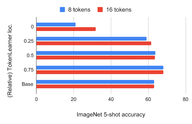
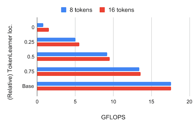
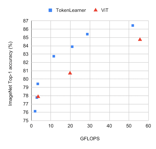
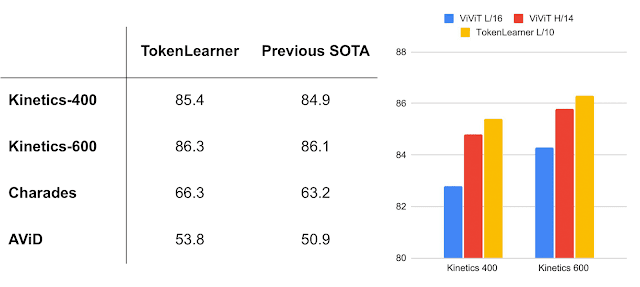
TokenLearner: Adaptive Space-Time Tokenization for Videos
Michael S. Ryoo, AJ Piergiovanni, Anurag Arnab, Mostafa Dehghani, Anelia Angelova
Towards Best-of-All-Worlds Online Learning with Feedback Graphs
Liad Erez, Tomer Koren
Training Over-Parameterized Models with Non-decomposable Objectives
Harikrishna Narasimhan, Aditya Krishna Menon
Twice Regularized MDPs and the Equivalence Between Robustness and Regularization
Esther Derman, Matthieu Geist, Shie Mannor
Unsupervised Learning of Compositional Energy Concepts
Yilun Du, Shuang Li, Yash Sharma, Joshua B. Tenenbaum, Igor Mordatch
User-Level Differentially Private Learning via Correlated Sampling
Badih Ghazi, Ravi Kumar, Pasin Manurangsi
ViSER: Video-Specific Surface Embeddings for Articulated 3D Shape Reconstruction
Gengshan Yang, Deqing Sun, Varun Jampani, Daniel Vlasic, Forrester Cole, Ce Liu*, Deva Ramanan
A Minimalist Approach to Offline Reinforcement Learning
Scott Fujimoto, Shixiang Gu
A Unified View of cGANs With and Without Classifiers
Si-An Chen, Chun-Liang Li, Hsuan-Tien Lin
CoAtNet: Marrying Convolution and Attention for All Data Sizes (see blog post)
Zihang Dai, Hanxiao Liu, Quoc V. Le, Mingxing Tan
Combiner: Full Attention Transformer with Sparse Computation Cost
Hongyu Ren*, Hanjun Dai, Zihang Dai, Mengjiao Yang, Jure Leskovec, Dale Schuurmans, Bo Dai
Contrastively Disentangled Sequential Variational Autoencoder
Junwen Bai, Weiran Wang, Carla P. Gomes
Controlling Neural Networks with Rule Representations
Sungyong Seo, Sercan O. Arik, Jinsung Yoon, Xiang Zhang, Kihyuk Sohn, Tomas Pfister
Dataset Distillation with Infinitely Wide Convolutional Networks
Timothy Nguyen*, Roman Novak, Lechao Xiao, Jaehoon Lee
Deep Synoptic Monte-Carlo Planning in Reconnaissance Blind Chess
Gregory Clark
Differentially Private Learning with Adaptive Clipping
Galen Andrew, Om Thakkar, Swaroop Ramaswamy, Hugh Brendan McMahan
Differentially Private Model Personalization
Prateek Jain, Keith Rush, Adam Smith, Shuang Song, Abhradeep Thakurta
Efficient Algorithms for Learning Depth-2 Neural Networks with General ReLU Activations
Pranjal Awasthi, Alex Tang, Aravindan Vijayaraghavan
Efficiently Identifying Task Groupings for Multi-Task Learning
Christopher Fifty, Ehsan Amid, Zhe Zhao, Tianhe Yu, Rohan Anil, Chelsea Finn
Generalized Shape Metrics on Neural Representations
Alex H. Williams, Erin Kunz, Simon Kornblith, Scott Linderman
High-Probability Bounds for Non-Convex Stochastic Optimization with Heavy Tails
Ashok Cutkosky, Harsh Mehta
Identity Testing for Mallows Model
Róbert Busa-Fekete, Dimitris Fotakis, Balázs Szörényi, Manolis Zampetakis
Learnable Fourier Features for Multi-dimensional Spatial Positional Encoding
Yang Li, Si Si, Gang Li, Cho-Jui Hsieh, Samy Bengio*
Learning to Select Exogenous Events for Marked Temporal Point Process
Ping Zhang, Rishabh K. Iyer, Ashish V. Tendulkar, Gaurav Aggarwal, Abir De
Meta-learning to Improve Pre-training
Aniruddh Raghu, Jonathan Peter Lorraine, Simon Kornblith, Matthew B.A. McDermott, David Duvenaud
Pointwise Bounds for Distribution Estimation Under Communication Constraints
Wei-Ning Chen, Peter Kairouz, Ayfer Özgür
REMIPS: Physically Consistent 3D Reconstruction of Multiple Interacting People Under Weak Supervision
Mihai Fieraru, Mihai Zanfir, Teodor Alexandru Szente, Eduard Gabriel Bazavan, Vlad Olaru, Cristian Sminchisescu
Replacing Rewards with Examples: Example-Based Policy Search via Recursive Classification
Benjamin Eysenbach, Sergey Levine, Ruslan Salakhutdinov
Revealing and Protecting Labels in Distributed Training
Trung Dang, Om Thakkar, Swaroop Ramaswamy, Rajiv Mathews, Peter Chin, Françoise Beaufays
Robust Predictable Control
Benjamin Eysenbach, Ruslan Salakhutdinov, Sergey Levine
Robust Visual Reasoning via Language Guided Neural Module Networks
Arjun Reddy Akula, Varun Jampani, Soravit Changpinyo, Song-Chun Zhu
Towards Understanding Retrosynthesis by Energy-Based Models
Ruoxi Sun, Hanjun Dai, Li Li, Steven Kearnes, Bo Dai
Exploring the Limits of Out-of-Distribution Detection
Stanislav Fort, Jie Ren, Balaji Lakshminarayanan
Minimax Regret for Stochastic Shortest Path
Alon Cohen, Yonathan Efroni, Yishay Mansour, Aviv Rosenberg
No Regrets for Learning the Prior in Bandits
Soumya Basu, Branislav Kveton, Manzil Zaheer, Csaba Szepesvari
Structured Denoising Diffusion Models in Discrete State-Spaces
Jacob Austin, Daniel D. Johnsonv, Jonathan Ho, Daniel Tarlow, Rianne van den Berg
The Sensory Neuron as a Transformer: Permutation-Invariant Neural Networks for Reinforcement Learning (see blog post)
Yujin Tang, David Ha
On the Existence of The Adversarial Bayes Classifier
Pranjal Awasthi, Natalie Frank, Mehyrar Mohri
Beyond Value-Function Gaps: Improved Instance-Dependent Regret Bounds for Episodic Reinforcement Learning
Christopher Dann, Teodor Vanislavov Marinov, Mehryar Mohri, Julian Zimmert
A Provably Efficient Model-Free Posterior Sampling Method for Episodic Reinforcement Learning
Christopher Dann, Mehryar Mohri, Tong Zhang, Julian Zimmert
Datasets & Benchmarks Accepted Papers
Reduced, Reused and Recycled: The Life of a Dataset in Machine Learning Research
Bernard Koch, Emily Denton, Alex Hanna, Jacob G. Foster
Datasets & Benchmarks Best Paper
Constructing a Visual Dataset to Study the Effects of Spatial Apartheid in South Africa
Raesetje Sefala, Timnit Gebru, Luzango Mfupe, Nyalleng Moorosi
AI and the Everything in the Whole Wide World Benchmark
Inioluwa Deborah Raji, Emily M. Bender, Amandalynne Paullada, Emily Denton, Alex Hannah
A Unified Few-Shot Classification Benchmark to Compare Transfer and Meta Learning Approaches
Vincent Dumoulin, Neil Houlsby, Utku Evci, Xiaohua Zhai, Ross Goroshin, Sylvain Gelly, Hugo Larochelle
The Neural MMO Platform for Massively Multi-agent Research
Joseph Suarez, Yilun Du, Clare Zhu, Igor Mordatch, Phillip Isola
Systematic Evaluation of Causal Discovery in Visual Model-Based Reinforcement Learning
Nan Rosemary Ke, Aniket Didolkar, Sarthak Mittal, Anirudh Goyal, Guillaume Lajole, Stefan Bauer, Danilo Rezende, Yoshua Bengio, Michael Mozer, Christopher Pal
STEP: Segmenting and Tracking Every Pixel
Mark Weber, Jun Xie, Maxwell Collins, Yukun Zhu, Paul Voigtlaender, Hartwig Adam, Bradley Green, Andreas Geiger, Bastian Leibe, Daneil Cremers, Aljosa Osep, Laura Leal-Taixe, Liang-Chieh Chen
Artsheets for Art Datasets
Ramya Srinivisan, Emily Denton, Jordan Famularo, Negar Rostamzadeh, Fernando Diaz, Beth Coleman
SynthBio: A Case in Human–AI Collaborative Curation of Text Datasets
Ann Yuan, Daphne Ippolito, Vitaly Niolaev, Chris Callison-Burch, Andy Coenen, Sebastian Gehrmann
Benchmarking Bayesian Deep Learning on Diabetic Retinopathy Detection Tasks
Neil Band, Tim G. J. Rudner, Qixuan Feng, Angelos Filos, Zachary Nado, Michael W. Dusenberry, Ghassen Jerfel, Dustin Tran, Yarin Gal
Brax – A Differentiable Physics Engine for Large Scale Rigid Body Simulation (see blog post)
C. Daniel Freeman, Erik Frey, Anton Raichuk, Sertan Girgin, Igor Mordatch, Olivier Bachem
MLPerf Tiny Benchmark
Colby Banbury, Vijay Janapa Reddi, Peter Torelli, Jeremy Holleman, Nat Jeffries, Csaba Kiraly, Pietro Montino, David Kanter, Sebastian Ahmed, Danilo Pau, Urmish Thakker, Antonio Torrini, Peter Warden, Jay Cordaro, Giuseppe Di Guglielmo, Javier Duarte, Stephen Gibellini, Videet Parekh, Honson Tran, Nhan Tran, Niu Wenxu, Xu Xuesong
Automatic Construction of Evaluation Suites for Natural Language Generation Datasets
Simon Mille, Kaustubh D. Dhole, Saad Mahamood, Laura Perez-Beltrachini, Varun Gangal, Mihir Kale, Emiel van Miltenburg, Sebastian Gehrmann
An Empirical Investigation of Representation Learning for Imitation
Xin Chen, Sam Toyer, Cody Wild, Scott Emmons, Ian Fischer, Kuang-Huei Lee, Neel Alex, Steven Wang, Ping Luo, Stuart Russell, Pieter Abbeel, Rohin Shah
Multilingual Spoken Words Corpus
Mark Mazumder, Sharad Chitlangia, Colby Banbury, Yiping Kang, Juan Manuel Ciro, Keith Achorn, Daniel Galvez, Mark Sabini, Peter Mattson, David Kanter, Greg Diamos, Pete Warden, Josh Meyer, Vijay Janapa Reddi
Workshops
4th Robot Learning Workshop: Self-Supervised and Lifelong Learning
Sponsor: Google
Organizers include Alex Bewley, Vincent Vanhoucke
Differentiable Programming Workshop
Sponsor: Google
Machine Learning for Creativity and Design
Sponsor: Google
Organizers include: Daphne Ippolito, David Ha
LatinX in AI (LXAI) Research @ NeurIPS 2021
Sponsor: Google
Sponsorship Level: Platinum
Workshop Chairs include: Andres Munoz Medina
Mentorship Roundtables include: Jonathan Huang, Pablo Samuel Castro
Algorithmic Fairness Through the Lens of Causality and Robustness
Organizers include: Jessica Schrouff, Awa Dieng
ImageNet: Past, Present, and Future
Organizers include: Lucas Beyer, Xiaohua Zhai
Speakers include: Emily Denton, Vittorio Ferrari, Alex Hanna, Alex Kolesnikov, Rebecca Roelofs
Optimal Transport and Machine Learning
Organizers include: Marco Cuturi
Safe and Robust Control of Uncertain Systems
Speakers include: Aleksandra Faust
CtrlGen: Controllable Generative Modeling in Language and Vision
Speakers include: Sebastian Gehrmann
Deep Reinforcement Learning
Organizers include: Chelsea Finn
Speakers include: Karol Hausam, Dale Schuurmans
Distribution Shifts: Connecting Methods and Applications (DistShift)
Speakers include: Chelsea Finn
ML For Systems
Organizers include: Anna Goldie, Martin Maas, Azade Nazi, Azalia Mihoseini, Milad Hashemi, Kevin Swersky
Learning in Presence of Strategic Behavior
Organizers include: Yishay Mansour
Bayesian Deep Learning
Organizers include: Zoubin Ghahramani, Kevin Murphy
Advances in Programming Languages and Neurosymbolic Systems (AIPLANS)
Organizers include: Disha Shrivastava, Vaibhav Tulsyan, Danny Tarlow
Ecological Theory of Reinforcement Learning: How Does Task Design Influence Agent Learning?
Organizers include: Shixiang Shane Gu, Pablo Samuel Castro, Marc G. Bellemare
The Symbiosis of Deep Learning and Differential Equations
Organizers include: Lily Hu
Out-of-Distribution Generalization and Adaptation in Natural and Artificial Intelligence
Speakers include: Chelsea Finn
Cooperative AI
Organizers include: Natasha Jaques
Offline Reinforcement Learning
Organizers include: Rishabh Agarwal, George Tucker
Speakers include: Minmin Chen
2nd Workshop on Self-Supervised Learning: Theory and Practice
Organizers include: Kristina Toutanova
Data Centric AI
Organizers include: Lora Aroyo
Math AI for Education (MATHAI4ED): Bridging the Gap Between Research and Smart Education
Organizers include: Yuhai (Tony) Wu
Tutorials
Beyond Fairness in Machine Learning
Organizers include: Emily Denton
Competitions
Evaluating Approximate Inference in Bayesian Deep Learning
Organizers include: Matthew D. Hoffman, Sharad Vikram
HEAR 2021 NeurIPS Challenge Holistic Evaluation of Audio Representations
Organizers include: Jesse Engel
Machine Learning for Combinatorial Optimization
Organizers include: Pawel Lichocki, Miles Lubin
*Work done while at Google. ↩
†Currently at Google. ↩

 GPU Operator 1.9 includes support NVIDIA DGX A100 systems with DGX OS and streamlined installation processes.