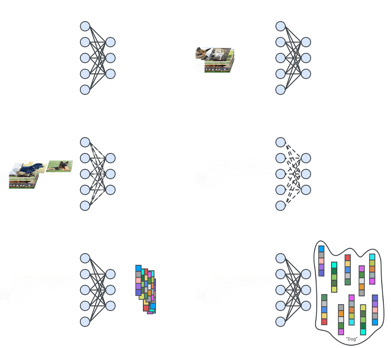
Today, we’re introducing luz, a high-level interface to torch that lets you train neural networks in a concise, declarative style. In some sense, it is to torch what Keras is to TensorFlow: It provides both a streamlined workflow and powerful ways for customization.
The time that it took to discover the COVID-19 vaccine is a testament to the pace of innovation in the healthcare industry. Pace of innovation can be directly linked to the thriving innovator ecosystem and the large number of AI-based healthcare startups. In comparison, the 5G wireless industry takes approximately a decade to introduce next … Continued
The time that it took to discover the COVID-19 vaccine is a testament to the pace of innovation in the healthcare industry. Pace of innovation can be directly linked to the thriving innovator ecosystem and the large number of AI-based healthcare startups. In comparison, the 5G wireless industry takes approximately a decade to introduce next generation systems.
The O-RAN Alliance is pioneering one way of addressing the pace of innovation and post-deployment feature enhancements. The traditional model of opaque design is being disrupted by a transparent paradigm with open and standardized interfaces. Forget using closed and proprietary interfaces, along with having limited options for an ecosystem to introduce new capabilities into deployed equipment.
The new paradigm includes concepts such as the RAN Intelligent Controller (RIC), a key technology that enables third parties to add new capabilities to the network. This provides monetization opportunities for not only the developer ecosystem but also network operators.
Future of wireless
Softwarization, virtualization, and disaggregation are some of the foundational concepts of 5G-and-beyond communication networks. Softwarization of the RAN, and its realization using a software-defined radio (SDR) paradigm, is critical for supporting the three key use cases that are the hallmark of 5G:
- Enhanced mobile broadband (eMBB)
- Ultra-reliable low-latency communication (URLLC)
- Massive machine type communication (mMTC)
A key differentiator between 4G and 5G is the capability, through software, to dynamically bring up and tear down network slices composed of eMBB, URLLC, and mMTC flows. Indeed, it’s a core value proposition of 5G.
Virtualization is an enabler for the efficient sharing of hardware and software assets in support of heterogeneous workloads in mobile edge computing (MEC). Disaggregation represents the dawn of a new ecosystem for the wireless industry. It opens the door to new business opportunities for a broad spectrum and a new generation of hardware developers.
Traditional, monolithic, opaque wireless infrastructure equipment is being disaggregated into the logical entities of the centralized unit (CU), distributed unit (DU), and radio unit (RU). This enables traditional network and emerging private 5G network operators with the flexibility to tailor a system architecture to meet their operational and business needs.
An equally important component of this new approach to wireless networking infrastructure is the standardization of interfaces, both physical and logical, between the hardware and software subsystems. Together with the development of an open software stack, these capabilities enable the rapid deployment of new network features through software. They also enable a new generation of software ecosystem developers to write application code for deployment in a network. These are applications that, by the virtue of these standardized interfaces and APIs, facilitate the control and interaction with entities running in the CU, DU, and RU.
RAN Intelligent Controller
The O-RAN Alliance is standardizing an open, intelligent, and disaggregated RAN architecture. The objective is to enable the construction of an operator-defined RAN using COTS hardware and provision for AI/ML-based intelligent control of 5G and future generation 6G wireless networks. Replace onventional RANs built using proprietary hardware, interfaces, and software with vRANs employing COTS hardware and open interfaces. The new architecture has options to support both proprietary software and applications developed by the ecosystem.
One of the most important elements of the O-RAN standard is the RAN Intelligent Controller (RIC) shown in Figure 1. The RIC consists of two main components:
- Non-real-time RIC (Non-RT RIC): Supports network functions at time scales of >1 second.
- Near real-time RIC (Near-RT RIC): Supports functions operating at time scales of 10 milliseconds–1 second.
As part of the SMO framework, some of the responsibilities of the Non-RT RIC include ML model lifecycle management and ML model selection. It also includes the marshaling, curation, and preprocessing of data gathered from the CU, DU, and even RU, in preparation for model training on the training host.
The Near-RT RIC introduced in the O-RAN architecture brings software-defined intelligence to the system. It includes advanced near-realtime analytics on data streamed from CU and DU, AI model inference, and online retraining of machine learning (ML) models.
Together, the SMO, Non-RT RIC, and Near-RT RIC bring ML techniques to all layers of the network architecture: layer-1 PHY, layer-2, and at the network level itself through AI-based self-organizing network (SoN) capabilities.

To help understand the RIC in more detail, consider an LTE example. The approach is similar for 5G NR. This example employs RIC-enabled AI for cell capacity management by using a long short-term memory (LSTM) traffic prediction model. The objective is to predict traffic for all cells in the network and mitigate future congestion. For more information, see Intelligent O-RAN for Beyond 5G and 6G Wireless Networks.
A two-layer LSTM network employs 12 LSTM cells per layer. It is trained using UE throughput measurements and physical resource block (PRB) utilization from 17 LTE eNBs in a real-world, fully operational, wireless network. The inference operation predicts UE throughput and eNB downlink PRB utilization 1 hour into the future.
Figure 2 shows the ground truth (actual) and predictions (LSTM inference) for throughput and PRB utilization for one cell of one eNB. The average prediction accuracy of 92.64% is remarkable. With the ability to forecast cell loadings at up to 1 hour into the future, the eNB can take steps to avoid coverage outages, for example cell splitting.

The role of the SMO in this example is to gather data from the O-CU/DU through the O1 interface (Figure 1) and deliver it to the Non-RT RIC. A Non-RT RIC rApp in turn queries the AI server associated with the SMO. The AI server runs a training process to update the LSTM model parameters based on fresh data collected from the operating network.
GPUs are the natural choice for ML training from both a programming model and compute capability perspective. The training workload is large due to the scale of the wireless network. We are not interested in model training for a single eNB with a few cells. Instead, we’re interested in training for a system that could have 100s to 1000s of base stations, with many 1000s of cells and 1000s to 10,000s of UEs. Having a GPU-powered AI training server provides the option of sharing that infrastructure over many SMO hosts. It is more cost– and power-efficient than a CPU AI training host. In other words, there are both CAPEX and OPEX advantages for the network operator.
After the training server has updated the LSTM model, the updated model parameters are returned to the Non-RT RIC rApp and the throughput/PRB prediction process continues with the updated model. Figure 3 shows the throughput gains. The vertical axis shows the fraction of the number of operating hours that user throughput for each band is indicated on the horizontal axis.
For example, you can see that, without cell splitting, throughput is in the range of 5-7.5 Mbps for approximately 1% of the time. With predictive cell splitting, throughput is in this same range for approximately 10%, a difference of a factor of 10.

An xApp that NVIDIA is researching is to enable intelligent and predictive multicell joint resource management. This has the potential to significantly improve the energy efficiency of the network.
AI algorithms running on a Non-RT RIC can predict user density and traffic load in each cell within a prediction window (on a seconds-to-minutes time scale). Predictions are based on the traffic history provided by CUs and DUs. Each DU scheduler makes decisions to switch off certain cells with low predicted traffic load to reduce energy consumption. They also trigger coordinated multipoint transmission/reception (CoMP) from neighboring active cells to ensure effective coverage.
The Near-RT RIC can help achieve the efficient multiplexing of eMBB and URLLC data traffic on the same frequency band. Due to significantly diverse service requirements, eMBB and URLLC transmissions are scheduled on two different time scales: time slot and mini-slot levels for eMBB and URLLC, respectively.
An AI-based xApp at the Near-RT RIC could learn and predict URLLC packet arrival patterns based on traffic statistics streamed from the DU over the E2 interface (Figure 1). Such predictive knowledge is used at the DU scheduler to optimize the resource reservation for URLLC mini-slots on top of eMBB data flows. It is also used to minimize the loss of eMBB throughput caused by such multiplexing.
You could also envision an xApp for massive MIMO beamforming optimization to maximize spectral efficiency. In this case, the Non-RT RIC hosts an rApp to perform long-term data analytics. The rApp’s task is to collect and analyze antenna array parameters and continually update an ML model. The Near-RT RIC xApp is implementing ML inference to configure, for example, beam horizontal and vertical aperture and cell shape.
Why GPUs?
The signal processing requirements (MACs/second) of the 5G NR physical layer are immense. The massive parallelism of the GPU brings the hardware resources to bear that can support this class of workload. In fact, a single GPU can support the baseband processing requirements of many 10s of carriers. Specialized hardware accelerators would typically have been employed in previous generation systems. However, the parallel nature of the GPU enables the softwarization of the RAN by providing a C++ abstraction for programming advanced signal-processing algorithms.
However, the value of the GPU extends beyond vRAN signal processing. In a 5G and 6G systems where big-data-meets-wireless, where AI/ML is used to improve network performance, GPUs are the default standard for model training and inference.
A common GPU-based hardware platform can support the tasks of training, inference, and signal processing. However, it’s not only about GPU hardware. An equally important consideration is the software for programming GPUs and SDKs and libraries for application development.
GPUs are programmed using CUDA, the world’s only commercially successful C/C++–based parallel programming framework. There is also a rich set of GPU libraries for developing, for example, data analytics pipelines using the NVIDIA RAPIDS software suite. The data analytics pipeline could be one of the services that the SMO/Non-RT RIC engages to update and fine-tune inference models running under the Near-RT RIC.
VMware and NVIDIA partnership
In early 2021, VMware released the world’s first O-RAN standard–compliant Near-RT RIC for integration and testing with select RAN and xApp vendor partners. To facilitate development of xApps on its Near-RT RIC, VMware provides its xApp partners with a set of developer resources packaged as an SDK.
Today, VMware and NVIDIA are excited to announce that the Near-RT RIC SDK now enables xApp developers to leverage GPU acceleration in their applications. This is an exciting milestone for the industry. It opens the doors for the larger industry to build AI/ML-powered capabilities for modern RANs, including those based on the NVIDIA Aerial gNB stack. Eventually, the VMware RIC and NVIDIA Aerial stack combination will enable the development and monetization of new and innovating xApps that enhance or expand the capabilities of a deployed network.
Conclusion
Openness and intelligence are the two core pillars of the O-RAN initiatives. As the 5G rollout and the ramp of 6G research continues, intelligence will be all-encompassing for the deployment, optimization, and operation of wireless networks.
Transitioning away from the opaque approach historically employed in cellular networks opens the door to a new era of swift innovation and time-to-market of new RAN features. NVIDIA vRAN (NVIDIA Aerial) and AI technology, combined with the VMware RIC, will foster a new generation of wireless and open up new monetization and innovation opportunities.
Virtualization is key to making networks flexible and data processing faster, better, and highly adaptive with network infrastructure from Core to RAN. You can achieve flexibility in deploying 5G services on commercial off-the-shelf (COTS) systems. However, 5G networks bring support for ultra-low latency, high-bandwidth applications, and scalable networks with network slicing and software defined networking … Continued
Virtualization is key to making networks flexible and data processing faster, better, and highly adaptive with network infrastructure from Core to RAN. You can achieve flexibility in deploying 5G services on commercial off-the-shelf (COTS) systems.
However, 5G networks bring support for ultra-low latency, high-bandwidth applications, and scalable networks with network slicing and software defined networking (SDN). 5G networks, especially virtualized RAN (vRAN), require both performance based on fast data processing and flexibility by virtualization at the same time.

The bottleneck of vRAN is the data processing in the PHY layer. Figure 2 shows the functional block diagram with the Option 7.2x architectural split. The PHY layer converts bits to radio waves in downlink by using various algorithms for scrambling, channel encoding, equalization, rate matching, and the reverse for uplink flow. Fronthaul interfaces with external radio units using the eCPRI protocol to reduce latency and jitter during data transfer.

GPU-based vRAN processing handles massive computations and heavy workloads without compromising on speed. The NVIDIA Aerial SDK is a cloud-native 5G vRAN solution running on NVIDIA GPUs to bring high performance computing (HPC) and signal processing all in one package.
Motivation for the benchmark of GPU-based vRAN
In addition to high speed and high-capacity communications, 5G technology is expected to offer low-latency transmission, offering more advanced signal processing. Because previous vRAN designs fail to deliver the communication performance anticipated for 5G, validation tests are being carried out with a view to boosting processing speed. SoftBank, along with NVIDIA, has been conducting such validation tests since 2019.
The NVIDIA Aerial SDK conforms to the standard specified by 3GPP and O-RAN Alliance, making this software highly compatible with the generalization and virtualization of 5G base stations. With in-line acceleration and software defined implementation, the performance improves with advances in GPUs while no design changes are required. Massive MIMO type communication being an integral part of RAN, NVIDIA Aerial can support higher bandwidths and data rates without sacrificing flexibility from virtualization.
To be precise, GPU performance is determined by its clock frequency and number of cores. These are virtualized by the CUDA C/C++ platform. The hardware structure is well hidden, and automatically schedules multiprocess operations to run with sufficient parallelism. If the Aerial SDK runs on different GPUs (GPUs with different numbers of cores), there is no need for additional development due to hardware changes. The advantages of the CUDA platform enable you to run the existing code on those GPUs without modification.
Softbank was interested in the flexibility of this GPU-based vRAN and collaborated with NVIDIA to conduct this validation to investigate the performance and features.
Performance testing conditions
In this test, signal processing was conducted to simulate uplink and downlink data communication for latency and power consumption. The benchmark was run on the server equipped with an NVIDIA V100 GPU (Figure 3).

Chipset | Intel Xeon CPU Platinum 8258(24 core 2.9GHz) |
Accelerator | 100 MHz |
Bandwidth | 100 MHz |
#MIMI layers | UL: 1-8 Layers DL: 1-16 |
Modulation | UL: 64 QAM DL: 256 QAM |
Tables 2 and 3 show the configuration details of the uplink and downlink test vectors.
Bandwidth (MHz) | 100 | 100 | 100 | 100 |
Cells | 1 | 2 | 4 | 8 |
Total Layers | 1 | 2 | 4 | 8 |
Total Users | 1 | 1 | 2 | 8 |
Layers per user | 1 | 2 | 2 | 2 |
Max length | 1 | 1 | 2 | 2 |
QAM | 64 | 64 | 64 | 64 |
Target code rate (R x 1024) | 948 | 948 | 948 | 948 |
Downlink Test Case 1 |
Downlink Test Case 2 |
Downlink Test Case 3 |
Donlink Test Case 4 |
|
Bandwidth (MHz) | 100 | 100 | 100 | 100 |
Cells | 1 | 1 | 1 | 1 |
Total layers | 2 | 4 | 8 | 16 |
Total users | 2 | 4 | 4 | 4 |
Layers per user | 1 | 1 | 2 | 4 |
max length | 1 | 1 | 2 | 2 |
QAM | 256 | 256 | 256 | 256 |
Target code rate (R x 1024) | 948 | 948 | 948 | 948 |
Results
The benchmark resulted in significant advantages in signal processing time and power consumption.
100MHz signal processing time
Figure 4 shows that GPU-based vRAN (NVIDIA Aerial) showed a remarkable advantage in processing time. The x-axis shows the total number of layers, and the y-axis shows the signal processing time. As the number of layers increases, the complexity of the signal processing increases. However, the increase in GPU latency for PHY processing is not proportional to the actual processing time required, making it more efficient for a higher number of layers.

This testing was limited to a single cell. Multicell performance on GPU parallel processors cannot be estimated from single cell performance, as the results would greatly underestimate the gains from processing additional cells in parallel.
For example, in the case of uplink, when the number of processed layers is increased from one layer to two layers, the processing time increases by only 1.18 times. SoftBank concluded that this is because the processing is performed efficiently by the massive parallel computing ability of the NVIDIA GPU. They also observed that the GPU can easily meet the 5G TTI budget with a single cell, so performant multicell processing would be within scope.
Power consumption
In Figure 5, the green bars represent the average power consumption of GPU card, and an error bar shows the range of GPU power consumption (representation from minimum power consumption to maximum power consumption). The x-axis shows the total number of layers (uplink) in the same way we showed the signal processing graph in the previous section. The y-axis shows the power consumption.
As explained earlier, as the number of layers increases, PHY processing becomes more computationally intensive, which puts more strain on the GPU. However, focusing on the average power consumption represented by the green bar, the increase in GPU power consumption is gradual, despite the increasing GPU load. It increases 1.41 times from one layer to two layers, and 1.56 times from one layer to four layers.

As the previously mentioned experiment showed, the power consumption of GPU-based vRAN demonstrated two important results:
- A rise in power consumption is not in proportion to the increase in the number of layers. This is going to be an advantage in case SoftBank deploys vRAN with a higher number of MIMO-layer configurations.
- Power consumption increased only when the GPU ran particular PHY signal processings. In other words, there is an evident correlation between GPU usage and the power consumption. This signifies that operators could cut down on the total power consumption if the vRAN system workload fluctuated a lot.
Importance of flexibility in deployment at edge
In 5G and beyond, we should expect the unexpected, especially when it comes to realizing new applications. In these potential applications, there will probably be some that require ultra-low latency to be meaningful, such as online gaming, AR/VR, and other typical MEC applications. You may not be able to put dedicated servers for these applications at edge, due to unavoidable limitations in terms of space, power draw, and other economic or engineering factors.
To tackle this type of adverse scenario, consider hosting latency-sensitive applications previously mentioned on a RAN system alongside 5GC functions necessary. This is the so-called “coexistence of 5G RAN and MEC” deployment scenario at which worldwide operators are aiming.

Because SoftBank is interested in the coexistence of 5G RAN and MEC, they are continuously verifying some applications using GPUs on MEC in parallel with this vRAN verification. For deployment scenarios that share resources at edge locations, they believe that there are some key requirements that cannot be ignored such as flexible programmability, cloud-native architecture, and proper multitenancy.
Through this vRAN validation, we confirmed the flexibility and high computational performance. Together with the fact that GPUs have a high affinity for AI processing, they felt that GPUs have an affinity for the coexistence of 5GRAN and MEC.
Because we both share the same views in the must-have edge requirements and ideal platforms in the future, SoftBank and NVIDIA are continuing to pursue this scenario in continuation of the successful vRAN benchmark.
Conclusion
Based on the key findings mentioned in this post, here are the conclusions SoftBank made in their GTC talk:
- RAN virtualization won’t stop. vRAN enables the adoption of open hardware with a software-defined RAN running on it, alongside other mobile capabilities such as MEC. These functional blocks are interconnected using open standard interfaces.
- Choose the right accelerator. To cope with computationally intensive PHY signal processing in open hardware platforms, you must choose the right accelerator. There are a couple of choices currently available on the market, GPU and others. The important factors to keep in mind are the hardware platform’s versatility, computing performance, cost, and its inherent programmability.
- GPUs are an ideal commercial vRAN solution in 5G networks. GPUs have valuable benefits, such as edge hardware resource sharing (MEC applications to be hosted on the same converged platform as gNB along with part of 5GC components) and its intrinsic programmability powered by CUDA.
- GPUs consume power proportionally. From time to time, the traffic to be processed by a gNB can be low. The way that GPUs consume power proportionally is beneficial in such cases, unlike other accelerators.
For more information, see the following resources:
- NVIDIA Aerial SDK
- [TITLE], SoftBank GTC webinar (Japanese/English)
Highlighting the growing importance of AI to innovation of all kinds in the U.K. and worldwide, NVIDIA founder and CEO Jensen Huang spoke today at the CogX conference. Huang was one of a trio of NVIDIA leaders appearing at the event hosted by Cognition X in King’s Cross, London, this week. “I believe artificial intelligence Read article >
The post NVIDIA CEO Speaks at UK AI Event on How AI Is Changing World appeared first on The Official NVIDIA Blog.
With the tech industry facing opportunities at every turn, it’s a ripe moment for NVIDIA’s acquisition of Arm, said CEOs of the companies in a frank conversation with a leading analyst. Patrick Moorhead of Moor Insights & Strategy posed tough questions and gave the deal a thumbs up in the session at the Six Five Read article >
The post NVIDIA, Arm CEOs Share Vision of a Deal Made for a Hypergrowth Era appeared first on The Official NVIDIA Blog.
How to install CuDNN on my PC?
I am using Nvidia GeForce Gt 1030 with the driver version 460.89! I have tried installing CUDA 11, CUDA 10.1 and CUDA 9 with all instructions followed. Still I get the error “CUDA_ERROR_LAUNCH_FAILED”. Please help!
submitted by /u/M-Groot
[visit reddit] [comments]
So I’m quite new to the world of Artificial Intelligence. I’m currently working on building a classification algorithm for raw data. This model will have 4 inputs, each a rank-1 tensor, but of different sizes. I could potentially make them all the same size if needed, but I would like to avoid this if possible. The output of the model would be a group number prediction based on softmax activation. My question is would it be better in terms of model accuracy to use the 4 arrays as separate inputs to a Functional model, or should I manipulate the arrays to all be the same size and create a Sequential model with one, rank-2 tensor as its input?
I apologize in advance if anything is poorly worded, or if there is necessary information missing. Please let me know if I can clarify anything.
submitted by /u/Tis98
[visit reddit] [comments]
In XGBoost 1.0, we introduced a new, official Dask interface to support efficient distributed training. Fast-forwarding to XGBoost 1.4, the interface is now feature-complete. If you are new to the XGBoost Dask interface, look at the first post for a gentle introduction. In this post, we look at simple code examples, showing how to maximize … Continued
In XGBoost 1.0, we introduced a new, official Dask interface to support efficient distributed training. Fast-forwarding to XGBoost 1.4, the interface is now feature-complete. If you are new to the XGBoost Dask interface, look at the first post for a gentle introduction. In this post, we look at simple code examples, showing how to maximize the benefits of GPU acceleration.
Our examples focus on the HIGGS dataset, a moderately sized classification problem from the UCI Machine Learning repository. In the following sections, we start from basic data loading and preprocessing with GPU-accelerated Dask and Dask-ml. Then, train an XGBoost model on returned data with different configurations. Also, share some new features along the way. After that, we showcase how to compute SHAP value on a GPU cluster and the speedup we can obtain. Lastly, we share some optimization techniques with inference.
The following examples need to be run on a machine with at least one NVIDIA GPU, which can be a laptop or a cloud instance. One of the advantages of Dask is its flexibility that users can test their code on a laptop. They can also scale up the computation to clusters with a minimum amount of code changes. Also, to set up the environment we need xgboost==1.4, dask, dask-ml, dask-cuda, and dask-cudf python packages, available from RAPIDS conda channels:
conda install -c rapidsai -c conda-forge dask[complete] dask-ml dask-cuda dask-cudf xgboost=1.4.2
Loading the data with Dask on a GPU cluster
First we download the dataset into the data
directory.
mkdir data
curl http://archive.ics.uci.edu/ml/machine-learning-databases/00280/HIGGS.csv.gz --output ./data/HIGGS.csv.gz
Then set up the GPU cluster using dask-cuda:
import os
from time import time
from typing import Tuple
from dask import dataframe as dd
from dask_cuda import LocalCUDACluster
from distributed import Client, wait
import dask_cudf
from dask_ml.model_selection import train_test_split
import xgboost as xgb
from xgboost import dask as dxgb
import numpy as np
import argparse
# … main content to be inserted here in the following sections
if __name__ == "__main__":
parser = argparse.ArgumentParser()
parser.add_argument("--n_workers", type=int, required=True)
args = parser.parse_args()
with LocalCUDACluster(args.n_workers) as cluster:
print("dashboard:", cluster.dashboard_link)
with Client(cluster) as client:
main(client)
Given a cluster, we start loading the data into GPUs. Because the data is loaded multiple times during parameter tuning, we convert the CSV file into Parquet format for better performance. This can be easily done using dask_cudf:
def to_parquet() -> str:
"""Convert the HIGGS.csv file to parquet files."""
dirpath = "./data"
parquet_path = os.path.join(dirpath, "HIGGS.parquet")
if os.path.exists(parquet_path):
return parquet_path
csv_path = os.path.join(dirpath, "HIGGS.csv")
colnames = ["label"] + ["feature-%02d" % i for i in range(1, 29)]
df = dask_cudf.read_csv(csv_path, header=None, names=colnames, dtype=np.float32)
df.to_parquet(parquet_path)
return parquet_path
After data loading, we prepare the training/validation splits:
def load_higgs(
path,
) -> Tuple[
dask_cudf.DataFrame, dask_cudf.Series, dask_cudf.DataFrame, dask_cudf.Series
]:
df = dask_cudf.read_parquet(path)
y = df["label"]
X = df[df.columns.difference(["label"])]
X_train, X_valid, y_train, y_valid = train_test_split(
X, y, test_size=0.33, random_state=42
)
X_train, X_valid, y_train, y_valid = client.persist(
[X_train, X_valid, y_train, y_valid]
)
wait([X_train, X_valid, y_train, y_valid])
return X_train, X_valid, y_train, y_valid
In the preceding example, we use dask-cudf for loading data from the disk, and the train_test_split function from dask-ml for splitting up the dataset. Most of the time, the GPU backend of dask works seamlessly with utilities in dask-ml and we can accelerate the entire ML pipeline.
Training with early stopping
One of the most frequently requested features is early stopping support for the Dask interface. In the XGBoost 1.4 release, not only can we specify the number of stopping rounds, but also develop customized early stopping strategies. For the simplest case, providing stopping rounds to the train function enables early stopping:
def fit_model_es(client, X, y, X_valid, y_valid) -> xgb.Booster:
early_stopping_rounds = 5
Xy = dxgb.DaskDeviceQuantileDMatrix(client, X, y)
Xy_valid = dxgb.DaskDMatrix(client, X_valid, y_valid)
# train the model
booster = dxgb.train(
client,
{
"objective": "binary:logistic",
"eval_metric": "error",
"tree_method": "gpu_hist",
},
Xy,
evals=[(Xy_valid, "Valid")],
num_boost_round=1000,
early_stopping_rounds=early_stopping_rounds,
)["booster"]
return booster
There are two things to notice in the preceding snippet. Firstly, we specify the number of rounds to trigger early stopping for training. XGBoost will stop the training process once the validation metric fails to improve in consecutive X rounds, where X is the number of rounds specified for early stopping. Secondly, we use a data type called DaskDeviceQuantileDMatrix for training but DaskDMatrix for validation. DaskDeviceQuantileDMatrix is a drop-in replacement of DaskDMatrix for GPU-based training inputs that avoids extra data copies.
DaskDeviceQuantileDMatrix can save a considerable amount of memory when used with gpu_hist and input data is already on GPU. Figure 1 depicts the construction of DaskDeviceQuantileDMatrix. Data partitions no longer need to be copied and concatenated, instead, a summary generated by the sketching algorithm is used as a proxy for the real data.

Inside XGBoost, early stopping is implemented as a callback function. The new callback interface can be used to implement more advanced early stopping strategies. The following code shows an alternative implementation of early stopping, with an additional parameter asking XGBoost to return only the best model instead of the full model:
def fit_model_customized_es(client, X, y, X_valid, y_valid): early_stopping_rounds = 5 es = xgb.callback.EarlyStopping(rounds=early_stopping_rounds, save_best=True) Xy = dxgb.DaskDeviceQuantileDMatrix(client, X, y) Xy_valid = dxgb.DaskDMatrix(client, X_valid, y_valid) # train the model booster = xgb.dask.train( client, { "objective": "binary:logistic", "eval_metric": "error", "tree_method": "gpu_hist", }, Xy, evals=[(Xy_valid, "Valid")], num_boost_round=1000, callbacks=[es], )["booster"] return booster
In the preceding example, the EarlyStopping callback is provided as an argument to train instead of using the early_stopping_rounds parameter. To provide a customized early stopping strategy, exploring other parameters of EarlyStopping or subclassing this callback is a great starting point.
Customized objective and evaluation metric
XGBoost is designed to be scalable through customized objective functions and metrics. In 1.4, this feature is brought to the dask interface. The requirement is exactly the same as for the single node interface:
def fit_model_customized_objective(client, X, y, X_valid, y_valid) -> dxgb.Booster:
def logit(predt: np.ndarray, Xy: xgb.DMatrix) -> Tuple[np.ndarray, np.ndarray]:
predt = 1.0 / (1.0 + np.exp(-predt))
labels = Xy.get_label()
grad = predt - labels
hess = predt * (1.0 - predt)
return grad, hess
def error(predt: np.ndarray, Xy: xgb.DMatrix) -> Tuple[str, float]:
label = Xy.get_label()
r = np.zeros(predt.shape)
predt = 1.0 / (1.0 + np.exp(-predt))
gt = predt > 0.5
r[gt] = 1 - label[gt]
le = predt
In the preceding function, we use the custom objective function and metric to implement a logistic regression model along with early stopping. Note that the function returns both gradient and hessian, which XGBoost uses to optimize the model. Also, the parameter named metric_name needs to be specified in our callback. It is used to inform XGBoost that the custom error function should be used for evaluating early stopping criteria.
Explaining the model
After obtaining our first model, we might want to explain predictions using SHAP. SHAP(SHapley Additive exPlanations) is a game theoretic approach to explain the output of machine learning models based on Shapley Value. For details about the algorithm, please refer to the papers. As XGBoost now has support for GPU-accelerated Shapley values, we extend this feature to the Dask interface. Now, users can compute shap values on distributed GPU clusters. This is enabled by the significantly improved predict function and the GPUTreeShap library:
def explain(client, model, X):
# Use array instead of dataframe in case of output dim is greater than 2.
X_array = X.values
contribs = dxgb.predict(
client, model, X_array, pred_contribs=True, validate_features=False
)
# Use the result for further analysis
return contribs
The performance of XGBoost computing shap value with multiple GPUs is shown in figure 2.

The benchmark is performed on an NVIDIA DGX-1 server with eight V100 GPUs and two 20-core Xeon E5–2698 v4 CPUs, with one round of training, shap value computation, and inference.
The resulting SHAP values can be used for visualization, tuning the column sampling with feature weights or for other data engineering purposes.
Running inference
After some tuning, we arrive at the final model for performing inference on new data. The prediction of the XGBoost Dask interface was not as efficient and also memory hungry in the older versions. In 1.4, we revised the predict function and added support for in-place prediction. For the normal prediction, it uses the same interface with shap value computation:
def predict(client, model, X):
predt = dxgb.predict(client, model, X)
assert isinstance(predt, dd.Series)
return predt
The standard predict function provides a general interface accepting both DaskDMatrix and dask collections (DataFrame or Array), but is not optimized for memory usage. Here, we replace it with in-place prediction, which supports basic inference task and doesn’t require copying the data into internal data structures of XGBoost:
def inplace_predict(client, model, X):
# Use inplace_predict instead of standard predict.
predt = dxgb.inplace_predict(client, model, X)
assert isinstance(predt, dd.Series)
return predt
The memory savings vary depending on the size of each chunk and the input types. When running inference multiple times with the same model, another potential optimization is prescattering the model. By default, XGBoost transfers the model to workers every time predict is called, incurring significant overhead. The good news is Dask functions accept a future object as a proxy to the finished model. We can then transfer data, which can overlap with other computations and persisting data on workers.
def inplace_predict_multi_parts(client, model, X_train, X_valid):
"""Simulate the scenario that we need to run prediction on multiple datasets using train
and valid. In real world the number of datasets is unlimited
"""
# prescatter the model onto workers
model_f = client.scatter(model)
predictions = []
for X in [X_train, X_valid]:
# Use inplace_predict instead of standard predict.
predt = dxgb.inplace_predict(client, model_f, X)
assert isinstance(predt, dd.Series)
predictions.append(predt)
return predictions
In the preceding snippet, we pass a future model to XGBoost instead of the real one. This way we avoid repeated transfers during prediction, or we can parallelize the model transfer with other operations like loading data, as suggested in the comments.
Putting it all together
In previous sections, we demonstrate early stopping, shap value computation, customized objective, and finally inference. The following chart shows the end-to-end speed-up for a GPU cluster with varying numbers of workers.

As before, the benchmark is performed on an NVIDIA DGX-1 server with eight V100 GPUs and two 20-core Xeon E5–2698 v4 CPUs, with one round of training, shap value computation, and inference. Also, we have shared two optimizations for memory usage and the overall memory usage comparison is depicted in Figure 4.

The left two columns are memory usage of training with a 64-bit data type, while the right two columns are training with a 32-bit data type. Standard means training using normal DaskDMatrix and predicts function. Efficient means using DaskDeviceQuantileDMatrix along with inplace_predict.
Scikit-learn wrapper
Previous sections consider basic model training with the ‘functional’ interface, however, there’s also a scikit-learn estimator-like interface. It’s easier to use but with some more constraints. In XGBoost 1.4, this interface has feature parity with the single node implementation. Users can choose different estimators like DaskXGBClassifier for classification and DaskXGBRanker for ranking. Check out the reference for a complete list of available estimators: https://xgboost.readthedocs.io/en/latest/python/python_api.html#module-xgboost.dask.
Summary
We have walked through an example of accelerating XGBoost on a GPU cluster with RAPIDS libraries showing that modernizing your XGBoost code can help maximize training efficiency. With the XGBoost Dask interface along with RAPIDS, users can achieve significant speedup with an easy-to-use API. Even though the XGBoost Dask interface has reached feature parity with single node API, development is continuing for better integration with other libraries for new features like hyperparameter tuning. For new feature requests relating to the dask interface, you can open an issue on XGBoost’s GitHub repository.
To learn more about using Dask and RAPIDS together, check out the NVIDIA presentations at the 2021 Dask Distributed Summit. For an overview of RAPIDS and Dask, listen into the GPU-accelerated Data Science workshop. For a deeper dive into code-based examples, check out the RAPIDS + Dask tutorial.
Audiences are making a round-trip to the moon with a science documentary that showcases China’s recent lunar explorations. Fly to the Moon, a series produced by the China Media Group (CMG) entirely in NVIDIA Omniverse, details the history of China’s space missions and shares some of the best highlights of the Chang ‘e-4 lunar lander, Read article >
The post Lunar Has It: Broadcasting Studio Uses NVIDIA Omniverse to Create Stunning Space Documentary appeared first on The Official NVIDIA Blog.
No need to hold out for a hero. You’ve made it to GFN Thursday. This year’s E3 was packed with news for GeForce NOW and we’re sharing the excitement from the announcements of Marvel’s Guardians of the Galaxy and Humankind. Both will join the GeForce NOW lineup when they launch later this year. On top Read article >
The post GFN Thursday Returns from E3 with Marvel’s Guardians of the Galaxy, Humankind Closed Beta and More appeared first on The Official NVIDIA Blog.