
|
submitted by /u/mad-myco [visit reddit] [comments] |

 DataBloom
|
|
submitted by /u/mad-myco [visit reddit] [comments] |
 DirectX 12 is a low-level programming API from Microsoft that reduces driver overhead in comparison to its predecessors. DirectX 12 provides more flexibility and fine-grained control on the underlying hardware using command queues, command lists, and so on, which results in better resource utilization. You can take advantage of these functionalities and optimize your applications … Continued
DirectX 12 is a low-level programming API from Microsoft that reduces driver overhead in comparison to its predecessors. DirectX 12 provides more flexibility and fine-grained control on the underlying hardware using command queues, command lists, and so on, which results in better resource utilization. You can take advantage of these functionalities and optimize your applications and get better performance over earlier DirectX versions. At the same time, the application, on its own, must take care of resource management, synchronization, and so on.
More and more game titles and other graphics applications are adopting DirectX12 APIs. Video Codec SDK 11.1 introduces DirectX 12 support for encoding on Windows 20H1 and later OS. This enables DirectX 12 applications to use NVENC across all generations of supported GPUs. The Video Codec SDK package contains NVENCODEAPI headers, sample applications demonstrating the usage, and the programming guide for using the APIs. The sample application contains C++ wrapper classes, which can be reused or modified as required.
typedef struct _NV_ENC_FENCE_POINT_D3D12
 {
     void*                   pFence; /**


The client application must also specify the input buffer format while initializing the NVENC.


Even though most of the parameters passed to the Encode picture API in DirectX 12 are same as those in other interfaces, there are certain functional differences. Synchronization at the input (the client application writing to the input surface and NVENC reading the input surface) and the output (NVENC writing the bitstream surface and the application reading it out) must be managed using fences. This is unlike previous DirectX interfaces, where it was automatically taken care by the OS runtime and driver.


In DirectX 12, additional information about fence and fence values are required as input parameters to the Encode picture API.  These fence and fence values are used to synchronize the CPU-GPU and GPU-GPU operations.  The application must send the following input and output struct pointers in NV_ENC_PIC_PARAMS::inputBuffer and NV_ENC_PIC_PARAMS:: outputBitstream, containing the fence and fence values:


typedef struct _NV_ENC_INPUT_RESOURCE_D3D12
 {
     NV_ENC_REGISTERED_PTR       pInputBuffer
     NV_ENC_FENCE_POINT_D3D12    inputFencePoint;
     …
 } NV_ENC_INPUT_RESOURCE_D3D12;

 typedef struct _NV_ENC_OUTPUT_RESOURCE_D3D12
 {
     NV_ENC_REGISTERED_PTR      pOutputBuffer;
     NV_ENC_FENCE_POINT_D3D12   outputFencePoint;
     …
 } NV_ENC_OUTPUT_RESOURCE_D3D12;
To retrieve the encoded output in asynchronous mode of operation, the application should wait on a completion event before calling NvEncLockBitstream. In the synchronous mode of operation, the application can call NvEncLockBitstream, as the NVENCODE API makes sure that encoding has finished before returning the encoded output. However, in both cases, the client application should pass a pointer to NV_ENC_OUTPUT_RESOURCE_D3D12, which was used in NvEncEncodePicture API, in NV_ENC_LOCK_BITSTREAM::outputBitstream.
For more information, see the Video Codec SDK programming guide. Encoder performance in DirectX 12 is close when compared to the other DirectX interfaces. The encoder quality is same across all interfaces.
 Using movies of living cancer cells, scientists create a convolutional neural network that can identify and predict aggressive metastatic melanomas.
Using a newly developed AI algorithm, researchers from the University of Texas Southwestern Medical Center are making early detection of aggressive forms of skin cancer possible. The study, recently published in Cell Systems, creates a deep learning model capable of predicting if a melanoma will aggressively spread, by examining cell features undetectable to the human eye.
“We now have a general framework that allows us to take tissue samples and predict mechanisms inside cells that drive disease, mechanisms that are currently inaccessible in any other way,” said senior author Gaudenz Danuser, the Patrick E. Haggerty Distinguished Chair in Basic Biomedical Science at the University of Texas Southwestern.
Melanoma—a serious form of skin cancer caused by changes in melanocyte cells— is the most likely of all skin cancers to spread if not caught early. Quickly identifying it helps doctors create effective treatment plans, and when diagnosed early, has a 5-year survival rate of about 99%.
Doctors often use biopsies, blood tests, or X-rays, CT, and PET scans to determine the stage of melanoma and whether it has spread to other areas of the body, known as metastasizing. Changes in cellular behavior could hint at the likelihood of the melanoma to spread, but they are too subtle for experts to observe.
The researchers thought using AI to help determine the metastatic potential of melanoma could be very valuable, but up until now AI models have not been able to interpret these cellular characteristics.
“We propose an algorithm that combines unsupervised deep learning and supervised conventional machine learning, along with generative image models to visualize the specific cell behavior that predicts the metastatic potential. That is, we map the insight gained by AI back into a data cue that is interpretable by human intelligence,” said Andrew Jamieson, study coauthor and assistant professor in bioinformatics at UT Southwestern.
Using tumor images from seven patients with a documented timeline of metastatic melanoma, the researchers compiled a time-lapse dataset of more than 12,000 single melanoma cells in petri dishes. Resulting in approximately 1,700,000 raw images, the researchers used a deep learning algorithm to identify different cellular behaviors.
Based on these features, the team then “reverse engineered’’ a deep convolutional neural network able to tease out the physical properties of aggressive melanoma cells and predict whether cells have high metastatic potential.
The experiments were run on the UT Southwestern Medical Center BioHPC cluster with CUDA-accelerated NVIDIA V100 Tensor Core GPUs. They trained multiple deep learning models on the 1.7 million cell images to visualize and explore the massive data set that started at over five TBs of raw microscopy data.
The researchers then tracked the spread of melanoma cells in mice and tested whether these specific predictors lead to highly metastatic cells. They found the cell types they’d classified as highly metastatic spread throughout the entire animal, while those classified low did not.
There is more work to be done before the research can be deployed in a medical setting. The team also points out that the study raises questions about whether this applies to other cancers, or if melanoma metastasis is an outlier.
“The result seems to suggest that the metastatic potential, at least of melanoma, is set by cell-autonomous rather than environmental factors,” Jamieson said.
Applications of the study could also go beyond cancer, and transform diagnoses of other diseases.
Read the full article in Cell Systems>>
Read more >>
 Modern graphics APIs, such as Direct3D 12 and Vulkan, are designed to provide relatively low-level access to the GPU and eliminate the GPU driver overhead associated with API translation. This low-level interface allows applications to have more control over the system and provides the ability to manage pipelines, shader compilation, memory allocations, and resource descriptors … Continued
Modern graphics APIs, such as Direct3D 12 and Vulkan, are designed to provide relatively low-level access to the GPU and eliminate the GPU driver overhead associated with API translation. This low-level interface allows applications to have more control over the system and provides the ability to manage pipelines, shader compilation, memory allocations, and resource descriptors in a way that is best for each application.
On the other hand, this closer-to-the-hardware access to the GPU means that the application must manage these things on its own, instead of relying on the GPU driver. A basic “hello world” program that draws a single triangle using these APIs can grow to a thousand lines of code or more. In a complex renderer, managing the GPU memory, descriptors, and so on, can quickly become overwhelming if not done in a systematic way.
If an application or an engine must work with more than one graphics API, it can be done in two ways:
NVIDIA Rendering Hardware Interface (NVRHI) is a library that handles these drawbacks. It defines a custom, higher-level graphics API that maps well to the three supported native graphics APIs: Vulkan, D3D12, and D3D11. It manages resources, pipelines, descriptors, and barriers in a safe and automatic way that can be easily disabled or bypassed when necessary to reduce CPU overhead. On top of that, NVRHI provides a validation layer that ensures that the application’s use of the API is correct, similar to what the Direct3D debug runtime or the Vulkan validation layers do, but on a higher level.
There are some features related to portability that NVRHI doesn’t provide. First, it doesn’t compile shaders at run time or read shader reflection data to bind resources dynamically. In fact, NVRHI doesn’t process shaders at run time at all. The application provides a platform-specific shader binary, that is, a DXBC, DXIL or SPIR-V blob. NVRHI passes that directly to the underlying graphics API. Matching the binding layouts is left up to the application and is validated by the underlying graphics API. Secondly, NVRHI doesn’t create graphics devices or windows. That is also left up to the application or other libraries, such as GLFW.
In this post, I go over the main features of NVRHI and explain how each feature helps graphics engineers be more productive and write safer code.
In Vulkan and D3D12, the application must take care to destroy only the device resources that the GPU is no longer using. This can be done with little overhead if the resource usage is planned carefully, but the problem is in the planning.
NVRHI follows the D3D11 resource lifetime model almost exactly. Resources, such as buffers, textures, or pipelines, have a reference count. When a resource handle is copied, the reference count is incremented. When the handle is destroyed, the reference count is decremented. When the last handle is destroyed and the reference count reaches zero, the resource object is destroyed, including the underlying graphics API resource. But that’s what D3D12 does as well, right? Not quite.
NVRHI also keeps internal references to resources that are used in command lists. When a command list is opened for recording, a new instance of the command list is created. That instance holds references to each resource it uses. When the command list is closed and submitted for execution, the instance is stored in a queue along with a fence or semaphore value that can be used to determine if the instance has finished executing on the GPU. The same command list can be reopened for recording immediately after that, even while the previous instance is still executing on the GPU.
The application should call the nvrhi::IDevice::runGarbageCollection method occasionally, at least one time per frame. This method looks at the in-flight command list instance queue and clears the instances that have finished executing. Clearing the instance automatically removes the internal references to the resources used in the instance. If a resource has no other references left, it is destroyed at that time.
This behavior can be shown with the following code example:
{
       // Create a buffer in a scope, which starts with reference count of 1
       nvrhi::BufferHandle buffer = device->createBuffer(...);

       // Creates an internal instance of the command list
       commandList->open();

       // Adds a buffer reference to the instance, which increases reference count to 2
       commandList->clearBufferUInt(buffer, 0);

       commandList->close();

       // The local reference to the buffer is released here, decrements reference count to 1
 }

 // Puts the command list instance into the queue
 device->executeCommandList(commandList);

 // Likely doesn't do anything with the instance
 // because it's just been submitted and still executing on the GPU
 device->runGarbageCollection();

 device->waitForIdle();

 // This time, the buffer should be destroyed because
 // waitForIdle ensures that all command list instances
 // have finished executing, so when the finished instance
 // is cleared, the buffer reference count is decremented to zero
 // and it can be safely destroyed
 device->runGarbageCollection();
The “fire and forget” pattern shown here, when the application creates a resource, uses it, and then immediately releases it, is perfectly fine in NVRHI, unlike D3D12 and Vulkan.
You might wonder whether this type of resource tracking becomes expensive if the application performs many draw calls with lots of resources bound for each draw call. Not really. Draw calls and dispatches do not deal with individual resources. Textures and buffers are grouped into immutable binding sets, which are created, hold permanent references to their resources, and are tracked as a single object.
So, when a certain binding set is used in a command list, the command list instance only stores a reference to the binding set. And that store is skipped if the binding set is already bound, so that repeated draw calls with the same bindings do not add tracking cost. I explain binding sets in more detail in the next section.
Another thing that can help reduce the CPU overhead imposed by resource lifetime tracking is the trackLiveness setting that is available on binding sets and acceleration structures. When this parameter is set to false, the internal references are not created for that particular resource. In this case, the application is responsible for keeping its own reference and not releasing it while the resource is in use.
NVRHI features a unique resource binding model designed for safety and runtime efficiency. As mentioned earlier, various resources that are used by graphics or compute pipelines are grouped into binding sets.
Put simply, a binding set is an array of resource views that are bound to particular slots in a pipeline. For example, a binding set may contain a structured buffer SRV bound to slot t1, a UAV for a single texture mip level bound to slot u0, and a constant buffer bound to slot b2. All the bindings in a set share the same visibility mask (which shader stages will see that binding) and register space, both dictated by the binding layout.
Binding layouts are the NVRHI version of D3D12 root signatures and Vulkan descriptor set layouts. A binding layout is like a template for a binding set. It declares what resource types are bound to which slots, but does not tell which specific resources are used.
Like the root signatures and descriptor set layouts, NVHRI binding layouts are used to create pipelines. A single pipeline may be created with multiple binding layouts. These can be useful to bin resources into different groups according to their modification frequency, or to bind different sets of resources to different pipeline stages.
The following code example shows how a basic compute pipeline can be created with one binding layout:
auto layoutDesc = nvrhi::BindingLayoutDesc()
     .setVisibility(nvrhi::ShaderType::All)
     .addItem(nvrhi::BindingLayoutItem::Texture_SRV(0))     // texture at t0
     .addItem(nvrhi::BindingLayoutItem::ConstantBuffer(2)); // constants at b2

// Create a binding layout.
nvrhi::BindingLayoutHandle bindingLayout = device->createBindingLayout(layoutDesc);

auto pipelineDesc = nvrhi::ComputePipelineDesc()
       .setComputeShader(shader)
       .addBindingLayout(bindingLayout);

// Use the layout to create a compute pipeline.
nvrhi::ComputePipelineHandle computePipeline = device->createComputePipeline(pipelineDesc);
Binding sets can only be created from a matching binding layout. Matching means that the layout must have the same number of items, of the same types, bound to the same slots, in the same order. This may look redundant, and the D3D12 and Vulkan APIs have less redundancy in their descriptor systems. This redundancy is useful: it makes the code more obvious, and it allows the NVRHI validation layer to catch more bugs.
auto bindingSetDesc = nvrhi::BindingSetDesc()
       // An SRV for two mip levels of myTexture.
       // Subresource specification is optional, default is the entire texture.
     .addItem(nvrhi::BindingSetItem::Texture_SRV(0, myTexture, nvrhi::Format::UNKNOWN,
       nvrhi::TextureSubresourceSet().setBaseMipLevel(2).setNumMipLevels(2)))
     .addItem(nvrhi::BindingSetItem::ConstantBuffer(2, constantBuffer));

// Create a binding set using the layout created in the previous code snippet.
nvrhi::BindingSetHandle bindingSet = device->createBindingSet(bindingSetDesc, bindingLayout);
Because the binding set descriptor contains almost all the information necessary to create the binding layout as well, it is possible to create both with one function call. That may be useful when creating some render passes that only need one binding set.
#include
...
nvrhi::BindingLayoutHandle bindingLayout;
nvrhi::BindingSetHandle bindingSet;
nvrhi::utils::CreateBindingSetAndLayout(device, /* visibility = */ nvrhi::ShaderType::All,
       /* registerSpace = */ 0, bindingSetDesc, /* out */ bindingLayout, /* out */ bindingSet);

// Now you can create the pipeline using bindingLayout.
Binding sets are immutable. When you create a binding set, NVRHI allocates the descriptors from the heap on D3D12 or creates a descriptor set on Vulkan and populates it with the necessary resource views.
Later, when the binding set is used in a draw or dispatch call, the binding operation is lightweight and translates to the corresponding graphics API binding calls. There is no descriptor creation or copying happening at render time.
Explicit barriers that change resource states and introduce dependencies in the graphics pipelines are an important part of both D3D12 and Vulkan APIs. They allow applications to minimize the number of pipeline dependencies and bubbles and to optimize their placement. They reduce CPU overhead at the same time by removing that logic from the driver. That’s relevant mostly to tight render loops that draw lots of geometry. Most of the time, especially when writing new rendering code, dealing with barriers is just annoying and bug-prone.
NVHRI implements a system that tracks the state of each resource and, optionally, subresource per command list. When a command interacts with a resource, the resource is transitioned into the state required for that command, if it’s not already in that state. For example, a writeTexture command transitions the texture into the CopyDest state, and a subsequent draw operation that reads from the texture transitions it into the ShaderResources state.
Special handling is applied when a resource is in the UnorderedAccess state for two consecutive commands: there is no transition involved, but a UAV barrier is inserted between the commands. It is possible to disable the insertion of UAV barriers temporarily, if necessary.
I said earlier that NVRHI tracks the state of each resource per command list. An application may record multiple command lists in any order or in parallel and use the same resource differently in each command list. Therefore, you can’t track the resource states globally or per-device because the barriers need to be derived while the command lists are being recorded. Global tracking may not happen in the same order as actual resource usage on the device command queue when the command lists are executed.
So, you can track resource states in each command list separately. In a sense, this can be viewed as a differential equation. You know how the state changes inside the command list, but you don’t know the boundary conditions, that is, which state each resource is in when you enter and exit the command list in their order of execution.
The application must provide the boundary conditions for each resource. There are two ways to do that:
beginTrackingTextureState and beginTrackingBufferState functions after opening the command list and the setTextureState and setBufferState functions before closing it.initialState and keepInitialState fields of the TextureDesc and BufferDesc structures when creating the resource. Then, each command list that uses the resource assumes that it’s in the initial state upon entering the command list, and transition it back into the initial state before leaving the command list.Here, you might wonder about avoiding the CPU overhead of resource state tracking, or manually optimizing barrier placement. Well, you can! The command lists have the setEnableAutomaticBarriers function that can completely disable automatic barriers. In this mode, use the setTextureState and setBufferState functions where a barrier is necessary. It still uses the same state tracking logic but potentially at a lower frequency.
NVRHI automates another aspect of modern graphics APIs that is often annoying to deal with. That’s the management of upload buffers and the tracking of their usage by the GPU.
Typically, when some texture or buffer must be updated from the CPU on every frame or multiple times per frame, a staging buffer is allocated whose size is multiple times larger than the resource memory requirements. This enables multiple frames in-flight on the GPU. Alternately, portions of a large staging buffer are suballocated at run time. It is possible to implement the same strategy using NVRHI, but there is a built-in implementation that works well for most use cases.
Each NVRHI command list has its own upload manager. When writeBuffer or writeTexture is called, the upload manager tries to find an existing buffer that is no longer used by the GPU that can fit the necessary data. If no such buffer is available, a new buffer is created and added to the upload manager’s pool. The provided data is copied into that buffer, and then a copy command is added to the command list. The tracking of which buffers are used by the GPU is performed automatically.
ConstantBufferStruct myConstants;
myConstants.member = value;

// This is all that's necessary to fill the constant buffer with data and have it ready for rendering.
commandList->writeBuffer(constantBuffer, myConstants, sizeof(myConstants));
The upload manager never releases its buffers, nor shares them with other command lists. Perhaps an application is doing a significant number of uploads, such as during scene loading, and then switching to a less upload-intensive mode of operation. In that case, it’s better to create a separate command list for the uploading activity and release it when the uploads are done. That releases the upload buffers associated with the command list.
It’s not necessary to wait for the GPU to finish copying data from the upload buffers. The resource lifetime tracking system described earlier does not release the upload buffers until the copies are done.
Sometimes, it is necessary to escape the abstraction layers and do something with the underlying graphics API directly. Maybe you have to use some feature that is not supported by NVRHI, demonstrate some API usage in a sample application, or make the portable rendering code work with a native resource coming from elsewhere. NVRHI makes it relatively easy to do these things.
Every NVRHI object has a getNativeObject function that returns an underlying API resource of the necessary type. The expected type is passed to that function, and it only returns a non-NULL value if that type is available, to provide some type safety.
Supported types include interfaces like ID3D11Device or ID3D12Resource and handles like vk::Image. In addition, the NVRHI texture objects have a getNativeView function that can create and return texture views, such as SRV or UAV.
For example, to issue some native D3D12 rendering commands in the middle of an NVRHI command list, you might use code like the following example:
ID3D12GraphicsCommandList* d3dCmdList = nvrhiCommandList->getNativeObject(
       nvrhi::ObjectTypes::D3D12_GraphicsCommandList);

D3D12_CPU_DESCRIPTOR_HANDLE d3dTextureRTV = nvrhiTexture->getNativeView(
       nvrhi::ObjectTypes::D3D12_RenderTargetViewDescriptor);

const float clearColor[4] = { 0.f, 0.f, 0.f, 0.f };
d3dCmdList->ClearRenderTargetView(d3dTextureRTV, clearColor, 0, nullptr);
The final productivity feature to mention here is the batch shader compiler that comes with NVRHI. It is an optional feature, and NVRHI can be completely functional without it. NVRHI accepts shaders compiled through other means. Still, it is a useful tool.
It is often necessary to compile the same shader with multiple combinations of preprocessor definitions. However, the native tools that Visual Studio provides for shader compilation, for example, do not make this task easy at all.
The NVRHI shader compiler solves exactly this problem. Driven by a text file that lists the shader source files and compilation options, it generates option permutations and calls the underlying compiler (DXC or FXC) to generate the binaries. The binaries for different versions of the same shader are then packaged into one file of a custom chunk-based format that can be processed using the functions declared in .
The application can load the file with all the shader permutations and pass it to nvrhi::utils::createShaderPermutation or nvrhi::utils::createShaderLibraryPermutation, along with the list of preprocessor definitions and their values. If the requested permutation exists in the file, the corresponding shader object is created. If it doesn’t, an error message is generated.
In addition to permutation processing, the shader compiler has other nice features. First, it scans the source files to build a tree of headers included in each one. It detects if any of the headers have been modified, and whether a particular shader must be rebuilt. Second, it can build all the outdated shaders in parallel using all available CPU cores.
In this post, I covered some of the most important features of NVRHI that, in my opinion, make it a pleasure to use. For more information about NVHRI, see the NVIDIAGameWorks/nvrhi GitHub repo, which includes a tutorial and a more detailed programming guide. The Donut Examples repository on GitHub has several complete applications written with NVRHI.
If you have questions about NVRHI, post an issue on GitHub or send me a message on Twitter (@more_fps).
The following python snippet
@tf.function def testfn(arr): if arr.size() == 0: raise ValueError('arr is empty') else: return tf.constant(True) arr = tf.TensorArray(tf.float32, 3) arr = arr.unstack([tf.constant(range(5), dtype=tf.float32) for i in range(3)]) tf.print('Size:', arr.size()) # "Size: 3" arrVal = testfn(arr) # Unexpected(?) ValueError: arr is empty
produces the following output
Size: 3 --------------------------------------------------------------------------- ValueError Traceback (...) ValueError: in user code: <ipython-input-72-47c594b1a619>:4 testfn * if arr.size() == 0: raise ValueError('arr is empty') ValueError: arr is empty
and I don’t understand why. When I print the size of the array I get 3. When I call testfn without the decorator, python also evaluates arr.size() to 3 in eager mode. But why does Autograph compile the array to something of size 0? And more importantly, how do I solve this problem? (I am very new to tensorflow)
submitted by /u/Dubmove
[visit reddit] [comments]
Don’t worry this bot is absolutely abysmal in online games if anyone tried to use it for this purpose. The detection is nowhere near as fast as human eye to finger reflex, even if you are a complete “noob”.
The reason I made this series is because not only was it fun and usual for me, maybe even uncharted territory as far as I am aware, but also I felt like it would be a fun way for young people to get started in learning about basic neural networks applied to computer vision.
The project includes two rather large datasets for CS:GO, one in 92×192 pixels and the other is 28×28 pixels. So if you are looking for unusual or “exotic” datasets to work with you may find this an interesting project.
The whole series can be found here:
https://james-william-fletcher.medium.com/list/fps-machine-learning-autoshoot-bot-for-csgo-100153576e93
It documents my journey through creating very basic neural networks in C and working my way up all the way to a CNN fully programmed and trained in C to then using a mixture of Tensorflow Keras and C. It covers many different aspects of working with neural networks, the intricacies of exporting Keras FNN into C and using Keras CNN models from C using a bridging daemon.
Maybe some of you will find it interesting or informative and I am always welcome to even the harshest of criticism.
submitted by /u/SirFletch
[visit reddit] [comments]
Let’s say you have a picture of a tic tac toe board after a game is done. I’m trying to make something that would be able to to translate the board to text.
I found this article which seemed to be pretty close but not exactly, also it’s not using Tensorflow.
My assumption is there would have to be some way to split the image into each of the nine different spaces, then check each space for either X,O, or BLANK. That’s the part I’m trying to wrap my head around. I’ve heard of stuff like image segmentation but not sure if that’s what I need.
Thanks!
submitted by /u/ThomasWaldick
[visit reddit] [comments]
SANTA CLARA, Calif., Aug. 19, 2021 (GLOBE NEWSWIRE) — NVIDIA will present at the following events for the financial community: BMO 2021 Technology Summit Tuesday, Aug. 24, at 10 a.m. Pacific …
 ‘Meet the Researcher’ is a series spotlighting researchers in academia who use NVIDIA technologies to accelerate their work. This month’s spotlight features Peerapon Vateekul, assistant professor at the Department of Computer Engineering, Faculty of Engineering, Chulalongkorn University (CU), Thailand. Vateekul drives collaboration activities between CU and the NVIDIA AI Technology Center (NVAITC) including seminars and workshops on … Continued
‘Meet the Researcher’ is a series spotlighting researchers in academia who use NVIDIA technologies to accelerate their work.
This month’s spotlight features Peerapon Vateekul, assistant professor at the Department of Computer Engineering, Faculty of Engineering, Chulalongkorn University (CU), Thailand. Vateekul drives collaboration activities between CU and the NVIDIA AI Technology Center (NVAITC) including seminars and workshops on joint applied research in Medical AI and NLP. He has been collaborating with NVIDIA since 2016 and became a university ambassador and certified DLI instructor for NVIDIA in 2018.
What are your research areas of focus?
My research focuses on interdisciplinary data analysis, applying machine learning techniques and a deep learning approach, to various domains. This includes AI-assisted medical diagnosis, hydrometeorology, geoinformatics, NLP, and finance. Some of my recent work focuses on medical diagnoses, such as working on AI-assisted solution polyp detection in colonoscopies in real time.
For NLP, my research group recently presented on a research project that deploys software agents equipped with natural language, understanding capabilities to read scholarly publications on the web.
When did you know that you wanted to be a researcher, that you wanted to pursue this field?
I realized that I wanted to be a researcher in the machine learning domain when I pursued my master’s degree. It was even clearer to me after I returned to Thailand and joined the Department of Computer Engineering at CU. I had the chance to collaborate with many researchers and professors from various schools. It felt impactful to be able to apply machine learning techniques to solve real-world problems.
What is the impact of your work on the field/community/world?
I tackle real world problems. AI-assisted telemedicine has played an important role in the pandemic era, thus I want to develop a model that can help a doctor to diagnose patients more accurately and efficiently.

For example, our research team is now implementing a real-time polyp detection solution for colonoscopies that can be deployed in an operation room. In this work, we have overcome the real-time inference constraint by using both software and hardware solutions. Especially for the hardware, where we have used a medical computer with an NVIDIA GeForce RTX, alongside a video switcher to analyze and render the video in real-time.
How do you use NVIDIA technology in your research?
I have been using NVIDIA technology in two aspects. First, a powerful server with an NVIDIA GPU is crucial to my research. Second, I have been using NVIDIA SDK’s and pretrained models from NVIDIA NGC in research works. For example, I have collaborated with Prof. Sira Sriswasdi from the medical school at CU. We aim to improve the COVID-19 diagnosis and prognosis prediction by using multi-zone lung segmentation in chest x-ray images. We’re using the NVIDIA CLARA SDK, which is a complete solution for AI-assisted medical that also contains federated learning to train a model across multiple sites (hospitals) without sharing sensitive patient data.
What’s next for your research?
The next step in my research is to translate the research work into a product (software) that can be used in a real-world scenario. Furthermore, I plan to extend my current works in many aspects. For example, I plan to extend the solution to support other parts of the gastrointestinal tracts. Apart from the polyp detection in colonoscopy, we can train a model to segment gastric intestinal metaplasia areas in gastroscopy.
Also, we are working to extend our scientific research system, ESRA, which now supports only publications in the computer science domain, to other domains, including bioinformatics.
Any advice for new researchers, especially to those who are inspired and motivated by your work?
For me, building successful research required three main factors: suitable machine learning techniques, training data along with domain experts, and a powerful GPU server. In addition, it is important to be a part of the research community since the AI related technologies have been changing rapidly; thus, you can keep updating your knowledge by being a part of the research community.
To learn more about the work that Peerapon Vateekul and his group is doing, visit his academia webpage.
 The Data Processing Unit, or DPU, has recently become popular in data center circles. But not everyone agrees on what tasks a DPU should perform or how it should do them. Idan Burstein, DPU Architect at NVIDIA, presents the applications and use cases that drive the architecture of the NVIDIA BlueField DPU.
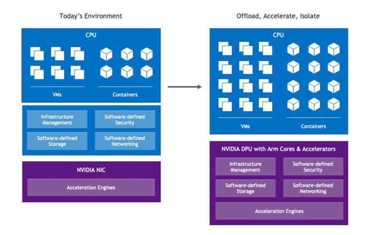
Today’s data centers are evolving rapidly and require new types of processors called data processing units (DPUs). The new requirements demand a specific type of DPU architecture, capable of offloading, accelerating, and isolating specific workloads. On August 23 at the Hot Chips 33 conference, NVIDIA silicon architect Idan Burstein discusses changing data center requirements and how they have driven the architecture of the NVIDIA BlueField DPU family.
Data centers today have changed from running applications in silos on dedicated server clusters. Now, resources such as CPU compute, GPU compute, and storage are disaggregated so that they can be composed (allocated and assembled) as needed. They are then recomposed (reallocated) as the applications and workloads change.
GPU-accelerated AI is becoming mainstream and enhancing myriad business applications, not just scientific applications. Servers that were primarily virtualized are now more likely to run in containers on bare metal servers, which still need software-defined infrastructure even though they no longer have a hypervisor or VMs. Cybersecurity tools such as firewall agents and anti-malware filters must run on every server to support a zero-trust approach to information security. These changes have huge consequences for the way networking, security, and management need to work, driving the need for DPUs in every server.
The best definition of the DPU’s mission is to offload, accelerate, and isolate infrastructure workloads.
A DPU should be able to do all three tasks.
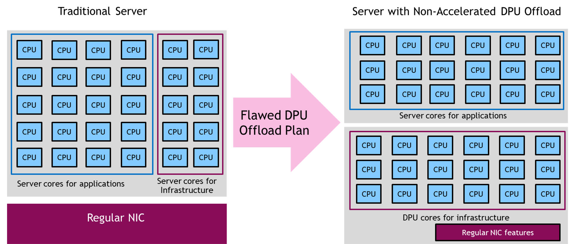
One approach tried by some DPU vendors is to place a large number of CPU cores on the DPU to offload the workloads from the server CPU. Whether these are Arm, RISC, X86, or some other type of CPU core, the approach is fundamentally flawed because the server’s CPUs or GPUs are already efficient for CPU-optimal or GPU-optimal workloads. While it’s true that Arm (or RISC or other) cores on a DPU might be more power efficient than a typical server CPU, the power savings are not worth the added complexity unless the Arm cores have an accelerator for that specific workload.
In addition, servers built on Arm CPUs are already available, for example, Amazon EC2 Graviton-based instances, Oracle A1 instances, or servers built on Ampere Computing’s Altra CPUs and Fujitsu’s A64FX CPUs. Applications that run more efficiently on Arm can already be deployed on server Arm cores. They should only be moved to DPU Arm cores if it’s part of the control plane or an infrastructure application that must be isolated from the server CPU.
Offloading a standard application workload from n number of server X86 cores to n or 2n Arm cores on a DPU doesn’t make technical or financial sense. Neither does offloading AI or serious machine learning workloads from server GPUs to DPU Arm cores. Moving workloads from a server’s CPU and GPU to the DPU’s CPU without any type of acceleration is at best a shell game and at worst decreases server performance and efficiency.
It’s clear that a proper DPU must use hardware acceleration to add maximum benefit to the data center. But what should it accelerate? The DPU is best suited for offloading workloads involving data movement, and security. For example, networking is an ideal task to offload to DPU silicon, along with remote direct memory access (RDMA), used to accelerate data movement between servers for AI, HPC, and big data, and storage workloads.
When the DPU has acceleration hardware for specific tasks, it can offload and run those with much higher efficiency than a CPU core. A properly designed DPU can perform the work of 30, 100, or even 300 CPU cores when the workload meets the DPU’s hardware acceleration capabilities.
The DPU’s CPU cores are ideal for running control plane or security workloads that must be isolated from the server’s application and OS domain. For example in a bare metal server, the tenants don’t want a hypervisor or VM running on their server to do remote management, telemetry, or security, because it hurts performance or may interfere with their applications. Yet the cloud operator still needs the ability to monitor the server’s performance and detect, block, or isolate security threats if they invade that server.
A DPU can run this software in isolation from the application domain, providing security and control while not interfering with the server’s performance or operations.
To learn more about how the NVIDIA BlueField DPU chip architecture meets the performance, security, and manageability requirements of modern data center, attend Idan Burstein’s session at Hot Chips 33. Idan explores what DPUs should offload or isolate. He explains what current and upcoming NVIDIA DPUs accelerate, allowing them to improve performance, efficiency, and security in modern data centers.