Edge computing is quickly becoming standard technology for organizations heavily invested in IoT, allowing organizations to process more data and generate better insights.
That’s over 100 IoT devices for every person on earth. The impact of this growth is amazing. As these devices continue to become smarter and more capable, organizations are finding creative new uses, as well as locations for these devices to operate.
Organizations have rallied around the power of vision to generate insights from IoT devices. Why?
Computer vision is a broad term for the work done with deep neural networks to develop human-vision capabilities for applications. It uses images and videos to automate tasks and generate insights. Devices, infrastructure, and spaces can leverage this power to enhance their perception, in much the same way the field of robotics has benefited from the technology.
While every computer vision setup is different, they all have one thing in common: they generate a ton of data. IDC predicts that IoT devices alone will generate over 90 zettabytes of data. The typical smart factory generates about 5 petabytes of video data per day and a smart city could generate 200 petabytes of data per day.
The sheer number of devices installed and the amount of data collected is putting a strain on traditional cloud and data center infrastructure. This is due to computer vision algorithms running in the cloud being unable to process data fast enough to return real-time insights. For many organizations, high-latency presents a significant safety concern.
Take the example of an autonomous forklift in a fulfillment center for a major retailer. The forklift uses a variety of sensors to perceive the world around it, making decisions off of the data it collects. It understands where it can and cannot drive, it can identify objects to move around the warehouse, and it knows when to stop abruptly to avoid colliding with a human worker in its path.
If the forklift sends data to the cloud, waits for it to be processed, and insights sent back to then act on, the forklift might not be able to stop in time to avoid a collision with a human worker.
In addition to latency concerns, sending the massive amount of data collected by IoT devices to the cloud to be processed is extremely costly. This high cost is why only 25% of IoT data gets analyzed*. 451 Research conducted a study in “Voice of the Enterprise: Internet of Things, Organizational Dynamics – Quarterly Advisory Report”where respondents admitted to only storing about half of all IoT data they create, and only analyzing about half of the data they store. By choosing not to process data due to high transit costs, organizations are neglecting valuable insights that could have a significant impact on their business.
These are some of the reasons why organizations have started using edge computing.
What is edge computing and its importance for IoT?
Edge computing is the concept of capturing and processing data as close to the source of the data as possible. This is done by deploying servers or other hardware to process data at the physical location of the IoT sensors. Since edge computing processes data locally—on the “edge” of a network, instead of in the cloud or a data center—it minimizes latency and data transit costs, allowing for real-time feedback and decision-making.
Edge computing allows organizations to process more data and generate more complete insights, which is why it is quickly becoming standard technology for organizations heavily invested in IoT. In fact, IDC reports that the edge computing market will be worth $34 billion by 2023.
Although the benefits of edge computing for AI applications using IoT are tangible, the combination of edge and IoT solutions has been an afterthought for many organizations. Ideally the convergence of these technologies is baked into the design, allowing the full potential of computer vision to be recognized, reaching new levels of automation and efficiency.
To learn more about how edge computing works and the benefits of edge computing, read the edge computing introduction post.
Editor’s Note: Watch the Analysing Cassandra Data using GPUs workshop. Organizations keep much of their high-speed transactional data in fast NoSQL data stores like Apache Cassandra®. Eventually, requirements emerge to obtain analytical insights from this data. Historically, users have leveraged external, massively parallel processing analytics systems like Apache Spark for this purpose. However, today’s analytics … Continued
Organizations keep much of their high-speed transactional data in fast NoSQL data stores like Apache Cassandra®. Eventually, requirements emerge to obtain analytical insights from this data. Historically, users have leveraged external, massively parallel processing analytics systems like Apache Spark for this purpose. However, today’s analytics ecosystem is quickly embracing AI and ML techniques whose computation relies heavily on GPUs.
In this post, we explore a cutting-edge approach for processing Cassandra SSTables by parsing them directly into GPU device memory using tools from the RAPIDS ecosystem. This will let users reach insights faster with less initial setup and also make it easy to migrate existing analytics code written in Python.
In this first post of a two-part series, we will take a quick dive into the RAPIDS project and explore a series of options to make data from Cassandra available for analysis with RAPIDS. Ultimately we will describe our current approach: parsing SSTable files in C++ and converting them into a GPU-friendly format, making the data easier to load into GPU device memory.
If you want to skip the step-by-step journey and try out sstable-to-arrow now, check out the second post.
What is RAPIDS
RAPIDS is a suite of open source libraries for doing analytics and data science end-to-end on a GPU. It emerged from CUDA, a developer toolkit developed by NVIDIA to empower developers to take advantage of their GPUs.
RAPIDS takes common AI / ML APIs like pandas and scikit-learn and makes them available for GPU acceleration. Data science, and particularly machine learning, uses numerous parallel calculations, which makes it better-suited to run on a GPU, which can “multitask” at a few orders of magnitude higher than current CPUs (image from rapids.ai):
Figure 1:
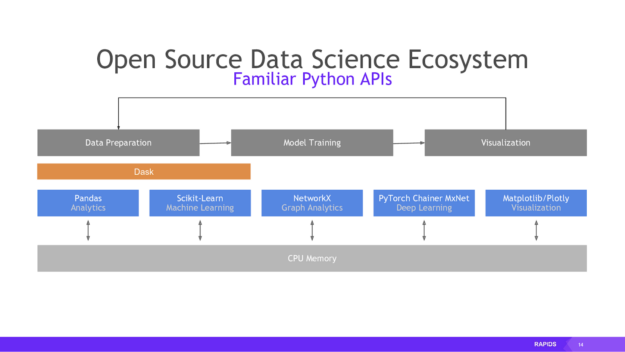
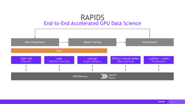
Once we get the data on the GPU in the form of a cuDF (essentially the RAPIDS equivalent of a pandas DataFrame), we can interact with it using an almost identical API to the Python libraries you might be familiar with, such as pandas, scikit-learn, and more, as shown in the images from RAPIDS below:
Figure 2:
Figure 3:
Note the use of Apache Arrow as the underlying memory format. Arrow is based on columns rather than rows, causing faster analytic queries. It also comes with inter-process communication (IPC) mechanism used to transfer an Arrow record batch (that is a table) between processes. The IPC format is identical to the in-memory format, which eliminates any extra copying or deserialization costs and gets us some extremely fast data access.
The benefits of running analytics on a GPU are clear. All you want is the proper hardware, and you can migrate existing data science code to run on the GPU simply by finding and replacing the names of Python data science libraries with their RAPIDS equivalents.
How do we get Cassandra data onto the GPU?
Over the past few weeks, I have been looking at five different approaches, listed in order of increasing complexity below:
Fetch the data using the Cassandra driver, convert it into a pandas DataFrame, and then turn it into a cuDF.
Same as the preceding, but skip the pandas step and transform data from the driver directly into an Arrow table.
Read SSTables from the disk using Cassandra server code, serialize it using the Arrow IPC stream format, and send it to the client.
Same as approach 3, but use our own parsing implementation in C++ instead of using Cassandra code.
Same as approach 4, but use GPU vectorization with CUDA while parsing the SSTables.
First, I will give a brief overview of each of these approaches, and then go through comparison at the end and explain our next steps.
Fetch data using the Cassandra driver
This approach is quite simple because you can use existing libraries without having to do too much hacking. We grab the data from the driver, setting session.row_factory to our pandas_factory function to tell the driver how to transform the incoming data into a pandas.DataFrame. Then, it is a simple matter to call the cudf.DataFrame.from_pandas function to load our data onto the GPU, where we can then use the RAPIDS libraries to run GPU-accelerated analytics.
The following code requires you to have access to a running Cassandra cluster. See the DataStax Python Driver docs for more info. You will also want to install the required Python libraries with Conda:
from cassandra.cluster import Cluster
from cassandra.auth import PlainTextAuthProvider

import pandas as pd
import pyarrow as pa
import cudf
from blazingsql import BlazingContext

import config

# connect to the Cassandra server in the cloud and configure the session settings
cloud_config= {
        'secure_connect_bundle': '/path/to/secure/connect/bundle.zip'
}
auth_provider = PlainTextAuthProvider(user=’your_username_here’, password=’your_password_here’)
cluster = Cluster(cloud=cloud_config, auth_provider=auth_provider)
session = cluster.connect()

def pandas_factory(colnames, rows):
    """Read the data returned by the driver into a pandas DataFrame"""
    return pd.DataFrame(rows, columns=colnames)
session.row_factory = pandas_factory

# run the CQL query and get the data
result_set = session.execute("select * from your_keyspace.your_table_name limit 100;")
df = result_set._current_rows # a pandas dataframe with the information
gpu_df = cudf.DataFrame.from_pandas(df) # transform it into memory on the GPU

# do GPU-accelerated operations, such as SQL queries with blazingsql
bc = BlazingContext()
bc.create_table("gpu_table", gpu_df)
bc.describe_table("gpu_table")
result = bc.sql("SELECT * FROM gpu_table")
print(result)
Fetch data using the Cassandra driver directly into Arrow
This step is identical to the previous one, except we can switch out pandas_factory with the following arrow_factory:
PythonCopy
def get_col(col):
    rtn = pa.array(col) # automatically detects the type of the array

    # for a full implementation, we would want to fully check which
arrow types want
    # to be manually casted for compatibility with cudf
    if pa.types.is_decimal(rtn.type):
        return rtn.cast('float32')
    return rtn

def arrow_factory(colnames, rows):
    # convert from the row format passed by
    # CQL into the column format of arrow
    cols = [get_col(col) for col in zip(*rows)]
    table = pa.table({ colnames[i]: cols[i] for i in
range(len(colnames)) })
    return table

session.row_factory = arrow_factory
We can then fetch the data and create the cuDF in the same way.
However, both of these two approaches have a major drawback: they rely on querying the existing Cassandra cluster, which we don’t want because the read-heavy analytics workload might affect the transactional production workload, where real-time performance is key.
Instead, we want to see if there is a way to get the data directly from the SSTable files on the disk without going through the database. This brings us to the next three approaches.
Read SSTables from the disk using Cassandra server code
Probably the simplest way to read SSTables on disk is to use the existing Cassandra server technologies, namely SSTableLoader. Once we have a list of partitions from the SSTable, we can manually transform the data from Java objects into Arrow Vectors corresponding to the columns of the table. Then, we can serialize the collection of vectors into the Arrow IPC stream format and then stream it in this format across a socket.
The code here is more complex than the previous two approaches and less developed than the next approach, so I have not included it in this post. Another drawback is that although this approach can run in a separate process or machine than the Cassandra cluster, to use SSTableLoader, we first want to initialize embedded Cassandra in the client process, which takes a considerable amount of time on a cold start.
Use a custom SSTable parser
To avoid initializing Cassandra, we developed our own custom implementation in C++ for parsing the binary data SSTable files. More information about this approach can be found in the next blog post. Here is a guide to the Cassandra storage engine by The Last Pickle, which helped a lot when deciphering the data format. We decided to use C++ as the language for the parser to anticipate eventually bringing in CUDA and also for low-level control to handle binary data.
Integrate CUDA to speed up table reads
We plan to start working on this approach once the custom parsing implementation becomes more comprehensive. Taking advantage of GPU vectorization should greatly speed up the reading and conversion processes.
Comparison
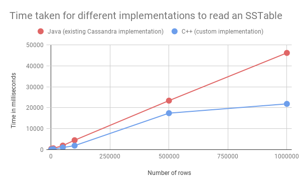
At the current stage, we are mainly concerned with the time it takes to read the SSTable files. For approaches 1 and 2, we can’t actually measure this time fairly, because 1) the approach relies on additional hardware (the Cassandra cluster) and 2). There are complex caching effects at play within Cassandra itself. However, for approaches 3 and 4, we can perform simple introspection to track how much time the program takes to read the SSTable file from start to finish.
Here are the results against datasets with 1k, 5K, 10k, 50k, 100k, 500k, and 1m rows of data generated by NoSQLBench:
Figure 4:
As the graph shows, the custom implementation is slightly faster than the existing Cassandra implementation, even without any additional optimizations such as multithreading.
Conclusion
Given that data access patterns for analytical use cases usually include large scans and often reading entire tables, the most efficient way to get at this data is not through CQL but by getting at SSTables directly. We were able to implement a sstable parser in C++ that can do this and convert the data to Apache Arrow so that it can be leveraged by analytics libraries including NVIDIA’s GPU-powered RAPIDS ecosystem. The resulting open-source (Apache 2 licensed) project is called sstable-to-arrow and it is available on GitHub and accessible through Docker Hub as an alpha release.
We will be holding a free online workshop, which will go deeper into this project with hands-on examples in mid-August! Sign up here if you are interested.
If you are interested in trying out sstable-to-arrow, look at the second blog post in this two-part series and feel free to reach out to seb@datastax.com with any feedback or questions.
I’ve deployed my own model with TF Serve in Docker. I’d like to consume that from a C# app via gRPC. So I guess I should somehow create the .proto files which to use to generate the C# classes. But how would I know the exact gRPC contract in order to create the .proto files?
The tech world this week gets its first look under the hood of the NVIDIA BlueField data processing unit. The chip invented the category of the DPU last year, and it’s already being embraced by cloud services, supercomputers and many OEMs and software partners. Idan Burstein, a principal architect leading our Israel-based BlueField design team, Read article >
This GFN Thursday brings in the highly anticipated magnum opus from SEGA and Amplitude Studios, HUMANKIND, as well as exciting rewards to redeem for members playing Eternal Return. There’s also updates on the newest Fortnite Season 7 game mode, “Impostors,” streaming on GeForce NOW. Plus, there are nine games in total coming to the cloud Read article >
NVIDIA researchers are presenting five papers on our groundbreaking research in speech recognition and synthesis at INTERSPEECH 2021.
Researchers from around the world working on speech applications are gathering this month for INTERSPEECH, a conference focused on the latest research and technologies in speech processing. NVIDIA researchers will present five papers on groundbreaking research in speech recognition and speech synthesis.
Conversational AI research is fueling innovations in speech processing that help computers communicate more like humans and add value to organizations.
Accepted papers from NVIDIA at this year’s INTERSPEECH features the newest speech technology advancements, from free fully formatted speech datasets to new model architectures that deliver state-of-the-art performance.
This talk will be live on Thursday, September 2, 2021 at 4:45 pm CET, 7:45 am PST
Compressing 1D Time-Channel Separable Convolutions Using Sparse Random Ternary Matrices Authors: Gonçalo Mordido, Matthijs Van Keirsbilck, Alexander Keller From the abstract: For command recognition on Google Speech Commands v1, we improve the state-of-the-art accuracy from 97.21% to 97.41% at the same network size. For speech recognition on Librispeech, we half the number of weights to be trained while only sacrificing about 1% of the floating-point baseline’s word error rate.
This talk will be live on Friday, September 3, 2021 at 4 pm CET, 7 am PST
NVIDIA today reported record revenue for the second quarter ended August 1, 2021, of $6.51 billion, up 68 percent from a year earlier and up 15 percent from the previous quarter, with record revenue from the company’s Gaming, Data Center and Professional Visualization platforms.
Hi. I’ve gone through a good deal of Geron’s HOML, but I feel like I’m lacking in the ‘basics’ of TensorFlow. Are there any good ‘pre-HOML’ resources that you can recommend to build a firmer foundation? Thanks!

 Edge computing is quickly becoming standard technology for organizations heavily invested in IoT, allowing organizations to process more data and generate better insights.
  Editor’s Note: Watch the Analysing Cassandra Data using GPUs workshop. Organizations keep much of their high-speed transactional data in fast NoSQL data stores like Apache Cassandra®. Eventually, requirements emerge to obtain analytical insights from this data. Historically, users have leveraged external, massively parallel processing analytics systems like Apache Spark for this purpose. However, today’s analytics …
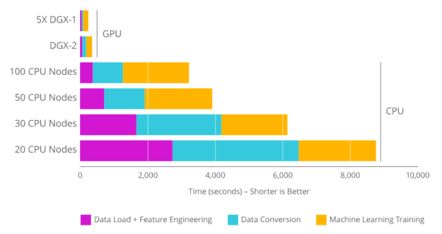
 NVIDIA researchers are presenting five papers on our groundbreaking research in speech recognition and synthesis at INTERSPEECH 2021.