
Using the torch just-in-time (JIT) compiler, it is possible to query a model trained in R from a different language, provided that language can make use of the low-level libtorch library. This post shows how. In addition, we try to untangle a bit of the terminological jumble surrounding the topic.
Any one knows difference between TimeDistributed(Conv1D) and TimeDistributed?
Example which caused confusion is here: https://stackoverflow.com/questions/68708007/difference-between-timedistributedconv1d-and-timedistributed
submitted by /u/give_me_the_truth
[visit reddit] [comments]
Data underlies much of machine learning (ML) research and development, helping to structure what a machine learning algorithm learns and how models are evaluated and benchmarked. However, data collection and labeling can be complicated by unconscious biases, data access limitations and privacy concerns, among other challenges. As a result, machine learning datasets can reflect unfair social biases along dimensions of race, gender, age, and more.
Methods of examining datasets that can surface information about how different social groups are represented within are a key component of ensuring development of ML models and datasets is aligned with our AI Principles. Such methods can inform the responsible use of ML datasets and point toward potential mitigations of unfair outcomes. For example, prior research has demonstrated that some object recognition datasets are biased toward images sourced from North America and Western Europe, prompting Google’s Crowdsource effort to balance out image representations in other parts of the world.
Today, we demonstrate some of the functionality of a dataset exploration tool, Know Your Data (KYD), recently introduced at Google I/O, using the COCO Captions dataset as a case study. Using this tool, we find a range of gender and age biases in COCO Captions — biases that can be traced to both dataset collection and annotation practices. KYD is a dataset analysis tool that complements the growing suite of responsible AI tools being developed across Google and the broader research community. Currently, KYD only supports analysis of a small set of image datasets, but we’re working hard to make the tool accessible beyond this set.
Introducing Know Your Data
Know Your Data helps ML research, product and compliance teams understand datasets, with the goal of improving data quality, and thus helping to mitigate fairness and bias issues. KYD offers a range of features that allow users to explore and examine machine learning datasets — users can filter, group, and study correlations based on annotations already present in a given dataset. KYD also presents automatically computed labels from Google’s Cloud Vision API, providing users with a simple way to explore their data based on signals that weren’t originally present in the dataset.
A KYD Case Study
As a case study, we explore some of these features using the COCO Captions dataset, an image dataset that contains five human-generated captions for each of over 300k images. Given the rich annotations provided by free-form text, we focus our analysis on signals already present within the dataset.
Exploring Gender Bias
Previous research has demonstrated undesirable gender biases within computer vision datasets, including pornographic imagery of women and image label correlations that align with harmful gender stereotypes. We use KYD to explore gender biases within COCO Captions by examining gendered correlations within the image captions. We find a gender bias in the depiction of different activities across the images in the dataset, as well as biases relating to how people of different genders are described by annotators.
The first part of our analysis aimed to surface gender biases with respect to different activities depicted in the dataset. We examined images captioned with words describing different activities and analyzed their relation to gendered caption words, such as “man” or “woman”. The KYD Relations tab makes it easy to examine the relation between two different signals in a dataset by visualizing the extent to which two signals co-occur more (or less) than would be expected by chance. Each cell indicates either a positive (blue color) or negative (orange color) correlation between two specific signal values along with the strength of that correlation.
KYD also allows users to filter rows of a relations table based on substring matching. Using this functionality, we initially probed for caption words containing “-ing”, as a simple way to filter by verbs. We immediately saw strong gendered correlations:
 |
| Using KYD to analyze the relationship between any word and gendered words. Each cell shows if the two respective words co-occur in the same caption more (up arrow) or less often (down arrow) than pure chance. |
Digging further into these correlations, we found that several activities stereotypically associated with women, such as “shopping” and “cooking”, co-occur with images captioned with “women” or “woman” at a higher rate than with images captioned with “men” or “man”. In contrast captions describing many physically intensive activities, such as “skateboarding”, “surfing”, and “snowboarding”, co-occur with images captioned with “man” or “men” at higher rates.
While individual image captions may not use stereotypical or derogatory language, such as with the example below, if certain gender groups are over (or under) represented within a particular activity across the whole dataset, models developed from the dataset risk learning stereotypical associations. KYD makes it easy to surface, quantify, and make plans to mitigate this risk.
 |
| An image with one of the captions: “Two women cooking in a beige and white kitchen.” Image licensed under CC-BY 2.0. |
In addition to examining biases with respect to the social groups depicted with different activities, we also explored biases in how annotators described the appearance of people they perceived as male or female. Inspired by media scholars who have examined the “male gaze” embedded in other forms of visual media, we examined the frequency with which individuals perceived as women in COCO are described using adjectives that position them as an object of desire. KYD allowed us to easily examine co-occurrences between words associated with binary gender (e.g. “female/girl/woman” vs. “male/man/boy”) and words associated with evaluating physical attractiveness. Importantly, these are captions written by human annotators, who are making subjective assessments about the gender of people in the image and choosing a descriptor for attractiveness. We see that the words “attractive”, “beautiful”, “pretty”, and “sexy” are overrepresented in describing people perceived as women as compared to those perceived as men, confirming what prior work has said about how gender is viewed in visual media.
 |
| A screenshot from KYD showing the relationship between words that describe attractiveness and gendered words. For example, “attractive” and “male/man/boy” co-occur 12 times, but we expect ~60 times by chance (the ratio is 0.2x). On the other hand, “attractive” and “female/woman/girl” co-occur 2.62 times more than chance. |
KYD also allows us to manually inspect images for each relation by clicking on the relation in question. For example, we can see images whose captions include female terms (e.g. “woman”) and the word “beautiful”.
Exploring Age Bias
Adults older than 65 have been shown to be underrepresented in datasets relative to their presence in the general population — a first step toward improving age representation is to allow developers to assess it in their datasets. By looking at caption words describing different activities and analyzing their relation to caption words describing age, KYD helped us to assess the range of example captions depicting older adults. Having example captions of adults in a range of environments and activities is important for a variety of tasks, such as image captioning or pedestrian detection.
The first trend that KYD made clear is how rarely annotators described people as older adults in captions detailing different activities. The relations tab also shows a trend wherein “elderly”, “old”, and “older” tend not to occur with verbs that describe a variety of physical activities that might be important for a system to be able to detect. Important to note is that, relative to “young”, “old” is more often used to describe things other than people, such as belongings or clothing, so these relations are also capturing some uses that don’t describe people.
 |
| The relationship between words associated with age and movement from a screenshot of KYD. |
The underrepresentation of captions containing the references to older adults that we examined here could be rooted in a relative lack of images depicting older adults as well as in a tendency for annotators to omit older age-related terms when describing people in images. While manual inspection of the intersection of “old” and “running” shows a negative relation, we notice that it shows no older people and a number of locomotives. KYD makes it easy to quantitatively and qualitatively inspect relations to identify dataset strengths and areas for improvement.
Conclusion
Understanding the contents of ML datasets is a critical first step to developing suitable strategies to mitigate the downstream impact of unfair dataset bias. The above analysis points towards several potential mitigations. For example, correlations between certain activities and social groups, which can lead trained models to reproduce social stereotypes, can be potentially mitigated by “dataset balancing” — increasing the representation of under-represented group/activity combinations. However, mitigations focused exclusively on dataset balancing are not sufficient, as our analysis of how different genders are described by annotators demonstrated. We found annotators’ subjective judgements of people portrayed in images were reflected within the final dataset, suggesting a deeper look at methods of image annotations are needed. One solution for data practitioners who are developing image captioning datasets is to consider integrating guidelines that have been developed for writing image descriptions that are sensitive to race, gender, and other identity categories.
The above case studies highlight only some of the KYD features. For example, Cloud Vision API signals are also integrated into KYD and can be used to infer signals that annotators haven’t labeled directly. We encourage the broader ML community to perform their own KYD case studies and share their findings.
KYD complements other dataset analysis tools being developed across the ML community, including Google’s growing Responsible AI toolkit. We look forward to ML practitioners using KYD to better understand their datasets and mitigate potential bias and fairness concerns. If you have feedback on KYD, please write to knowyourdata-feedback@google.com.
Acknowledgements
The analysis and write-up in this post were conducted with equal contribution by Emily Denton, Mark Díaz, and Alex Hanna. We thank Marie Pellat, Ludovic Peran, Daniel Smilkov, Nikhil Thorat and Tsung-Yi for their contributions to and reviews of this post.

Categories
Deciphering Ancient Texts with AI
 Using machine learning and visual psychophysics, researchers are developing AI models capable of transcribing ancient manuscripts.
Looking to reveal secrets of days past, historical scholars across the globe spend their life’s work translating ancient manuscripts. A team at the University of Notre Dame looks to help in this quest, with a newly developed machine learning model for translating and recording handwritten documents centuries old.
Using digitized manuscripts from the Abbey Library of Saint Gall, and a machine learning model that takes into account human perception, the study offers a notable improvement in the capabilities of deep learning transcription.
“We’re dealing with historical documents written in styles that have long fallen out of fashion, going back many centuries, and in languages like Latin, which are rarely ever used anymore. You can get beautiful photos of these materials, but what we’ve set out to do is automate transcription in a way that mimics the perception of the page through the eyes of the expert reader and provides a quick, searchable reading of the text,” Walter Scheirer, senior author and an associate professor at Notre Dame said in a press release.
Founded in 719, the Abbey Library of Saint Gall holds one of the oldest and richest library collections in the world. The library houses approximately 160,000 volumes and 2,000 manuscripts, dating back to the eighth century. Hand-written on parchment paper in languages rarely used today, many of these materials have yet to be read—a potential fortune of historical archives, waiting to be unearthed.
Machine learning methods capable of automatically transcribing these types of historical documents have been in the works, however challenges remain.
Up until now, large datasets have been necessary to boost the performance of these language models. With the vast number of volumes available, the work takes time, and relies on a relatively small number of expert scholars for annotation. Missing knowledge, such as the Medieval Latin dictionary that has never been compiled, poses even greater obstacles.
The team combined traditional machine learning methods with the science of visual psychophysics, which studies the relationship between the physical world and human behavior, to create more information-rich annotations. In this case, they incorporated the measurements of human vision into the training process of the neural networks when processing the ancient texts.
“It’s a strategy not typically used in machine learning. We’re labeling the data through these psychophysical measurements, which comes directly from psychological studies of perception—by taking behavioral measurements. We then inform the network of common difficulties in the perception of these characters and can make corrections based on those measurements,” Scheirer said.
To train, validate, and test the models the researchers used a set of digitized handwritten Latin manuscripts from St. Gall dating back to the ninth century. They asked experts to read and enter manual transcriptions from lines of text into custom designed software. Measuring the time for each transcription, gives insight into the difficulty of words, characters, or passages. According to the authors, this data helps reduce errors in the algorithm and provides more realistic readings.
All of the experiments were run using the cuDNN-accelerated PyTorch deep learning framework and GPUs. “We definitely could not have accomplished what we did without NVIDIA hardware and software,” said Scheirer.
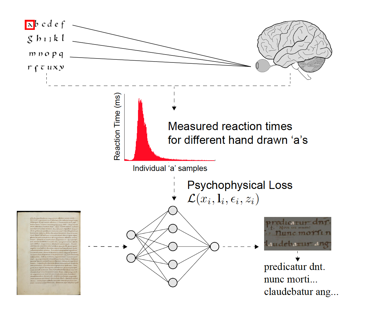
The research introduces a novel loss formulation for deep learning that incorporates measurements of human vision, which can be applied to different processing pipelines for handwritten document transcription. Credit: Scheirer et al/IEEE
There are still areas the team is working to improve. Damaged and incomplete documents, along with illustrations and abbreviations pose a special challenge for the models.
“The inflection point AI reached thanks to Internet-scale data and GPU hardware is going to benefit cultural heritage and the humanities just as much as other fields. We’re just scratching the surface of what we can do with this project,” said Scheirer.
Read the full article in IEEE Transactions on Pattern Analysis and Machine Intelligence >>
Read more >>
Talk about a signal boost. Creative Technology is tackling 4K and 8K signals, as well as new broadcast workflows, with the latest NVIDIA networking technologies. The London-based firm is one of the world’s leading suppliers of audio visual equipment for broadcasting and online events. Part of global production company NEP Group, CT helps produce high-quality Read article >
The post On the Air: Creative Technology Elevates Broadcast Workflows for International Sporting Event with NVIDIA Networking appeared first on The Official NVIDIA Blog.
Categories
NVIDIA-Certified Systems Land on the Desktop
Enterprises challenged with running accelerated workloads have an answer: NVIDIA-Certified Systems. Available from nearly 20 global computer makers, these servers have been validated for running a diverse range of accelerated workloads with optimum performance, reliability and scale. Now NVIDIA-Certified Systems are expanding to the desktop with workstations that undergo the same testing to validate their Read article >
The post NVIDIA-Certified Systems Land on the Desktop appeared first on The Official NVIDIA Blog.
 This post discussing pros and cons of distinct memory layouts as well as memory pools for asynchronous memory allocation to enable zero-copy functionality.
Introduction
Efficient pipeline design is crucial for data scientists. When composing complex end-to-end workflows, you may choose from a wide variety of building blocks, each of them specialized for a dedicated task. Unfortunately, repeatedly converting between data formats is an error-prone and performance-degrading endeavor. Let’s change that!
In this post series, we discuss different aspects of efficient framework interoperability:
- We start with this post discussing pros and cons of distinct memory layouts as well as memory pools for asynchronous memory allocation to enable zero-copy functionality.
- In the second post, we highlight bottlenecks occurring during data loading/transfers and how to mitigate them using Remote Direct Memory Access (RDMA) technology.
- In the third post, we dive into the implementation of an end-to-end pipeline demonstrating the discussed techniques for optimal data transfer across data science frameworks.
To learn more on framework interoperability, check out our presentation at NVIDIA’s GTC 2021 Conference.
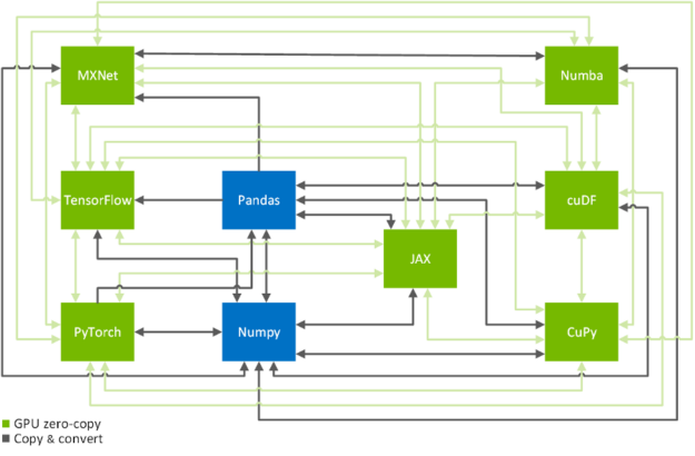
Zero-copy functionality is a crucial technique to efficiently copy data across GPU-accelerated data science frameworks: TensorFlow, PyTorch, MXNet, cuDF, CuPy, Numba, and JAX (see Figure 2). In the following, we will show you how to achieve that in a systematic manner. If you are only here to look up the commands on how to transfer data from one framework to another, you might want to have a look at this conversion table.
Memory layouts, data formats and memory pools
Memory Layouts
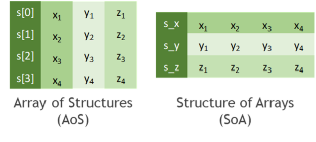
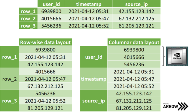
Before we start talking about how to copy data efficiently, let’s discuss how to store tabular data. In practice, all data formats inherit from one of the two major memory layouts known to computer scientists (see Figure 3):
- Array of Structures (AoS): A sequence of one or more data points x, y, z, … of potentially distinct type is represented as a structure S. Several instances of those data points are allocated as an array s of the new data type S. The original list of points x, y, z, … of the k-th instance is then accessed through the members s[k].x, s[k].y, s[k].z, … of the struct instance s[k].
- Structure of Arrays (SoA): Several instances of data points x, y, z, … are stored in separated arrays s_x, s_y, s_z, … The original points x, y, z, … of the k-th instance are then accessed by s_x[k], s_y[k], s_z[k], … Finally, these arrays can be interpreted as a single instance of a (merely virtually existing) structure, hence the name SoA.
While the AoS layout looks more structured (pun intended) than SoA from a programmatic and abstraction point of view, it tends to be less suited for massively parallel algorithms in terms of achievable performance. This can be explained by a less efficient utilization of cache lines when consistently accessing a subset of the structure members, for example, during the reduction of values along one coordinate axis. You can even find cases in the literature where on-the-fly AoS-to-SoA conversion can significantly improve performance compared to plain processing in an AOS memory layout.
The SoA memory layout exhibits further advantages when copying coordinate-slices of the data. Assume you want to transfer all the x-coordinates at once, then you can access the corresponding array without the time-consuming slicing of members in the AoS layout. Even better, one can avoid allocating auxiliary memory when transferring data by simply exposing the address of the array in memory without copying a single byte. Apache Arrow is built on top of this methodology: storing data of distinct data types in different arrays for the discussed reasons (see Figure 4). Note that mainstream data science frameworks treat the entries of an array in the SoA layout as if they were stored in columns instead of rows, as depicted in Figure 3. However, this is merely a convention as we all know that virtually all memory is linearly ordered.
Data formats and zero-copy mechanism
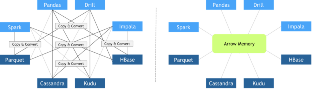
In recent years, different libraries have been developed to address different needs. At the same time, data science pipelines have become more and more complex, requiring the usage of multiple libraries to accomplish a wide variety of tasks. Unfortunately, when these libraries were designed, interoperability between frameworks was not conceived as a top priority. As a result, there was a lack of standardized data formats suitable for data science tasks. Some people were concerned about data standards at that moment, like Wes McKinney, creator of the pandas project. In 2011, he published this post about a future roadmap for rich scientific data structures in Python.
Since every library implemented its custom in-memory data layout and file formats, expensive copy-and-convert operations had to be performed when these libraries needed to collaborate. It was quite common that a significant portion of the total execution time was invested in meaningless copy-and-convert operations.
In October 2016, Apache Foundation released Arrow, a language-independent columnar-wise data format specification meant to deal efficiently with flat and hierarchical data on both CPUs and GPUs. Since then, many different frameworks have adopted it, facilitating zero-copy data exchange among them. Other key features of Apache Arrow columnar data format include:
- O(1) (constant-time) random access
- SIMD and vectorization-friendly
- Data adjacency for sequential access (scans)
- Relocatable without “pointer swizzling”, allowing for true zero-copy access in shared memory
Zero-copy mechanisms avoid unnecessary data transfers, reducing your application execution time drastically. Data science frameworks have added support to one or more of the following data formats: DLPack, CUDA Array Interface, and NumPy Array Interface.
DLPack is an open in-memory tensor structure for sharing tensors among frameworks. CUDA Array Interface and Numpy Array Interface are the de facto standards to exchange GPU and CPU array-like objects.
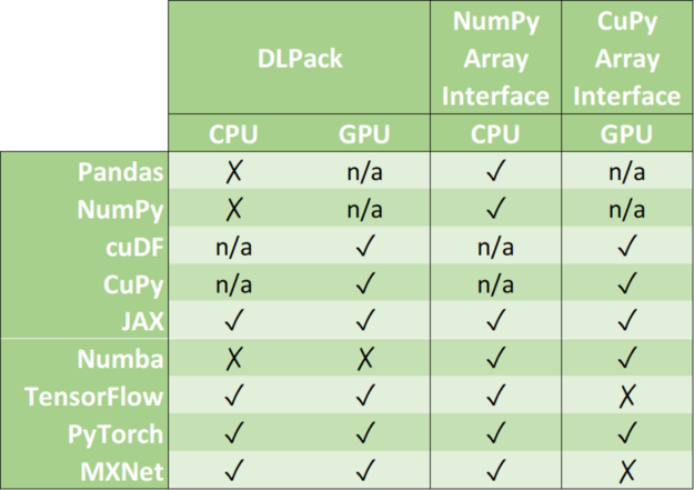
Please, note that some libraries like cuDF and CuPy exclusively run on GPU devices. Although it is possible to convert a NumPy array into a cuDF or CuPy object, we have marked its support as n/a because it requests data movement between host memory (CPU) and device memory (GPU).
In the following, we address memory layouts of the associated data objects in various frameworks, the efficient conversion of data objects using zero-copy, as well as the usage of a joint memory pool when mixing frameworks.
Memory pools
Memory allocations are expensive. They often impose global barriers, which block the remaining operations until the allocation is accomplished. Hence, repeatedly allocating memory in tight for-loops such as during the training of neural networks is prohibitive from a performance point of view. Modern data science and deep learning frameworks address this with dedicated memory pools. It is either preallocating a huge chunk of memory at the beginning of the program (for example, TensorFlow) or incrementally growing the pool using a few infrequent allocations (for example, PyTorch). Then, the preallocated memory is reused in a smart way by asynchronously assigning and retracting subsets of this memory range to/from whomever requests it. As an example, the RAPIDS Memory Manager (RMM) is a memory pool originally written for the RAPIDS data science framework. RMM facilitates blazingly fast host and device memory allocations. Mark Harris quantified the impact of RMM in this post: “We centralized memory management in cuDF by replacing all calls to cudaMalloc and cudaFree with RMM allocations. This was a lot of work, but it paid off. RMM calls are on the order of 1,000 times faster than cudaMalloc and cudaFree. The result was a 10x speedup for the mortgage demo.”
Several library-specific memory pools might compete for the same video RAM when combining distinct data science libraries. A straightforward workaround would be to limit the capacity of each memory pool to a fixed partition of the available memory. A better solution would be to use the same memory pool for all frameworks. Note that this does not necessarily mean that all frameworks must agree on the same memory pool implementation being shipped in their vanilla release. It is sufficient that all vendors agree to use an External Allocator Interface (EAI) for requesting and freeing memory in their frameworks.
void* allocate(std::size_t bytes, cudaStream_t stream)
void deallocate(void* p, std::size_t bytes, cudaStream_t stream)
Further advantages of an EAI are straightforward logging functionality, memory leak checking, as well as rate or resource limiting capabilities. For instance, the RAPIDS Memory Manager leverages unified memory to transparently oversubscribe GPU memory. The former translates into significantly reducing the chances of facing an Out of Memory error when working with huge datasets that do not fit in GPU memory.
The good news is that you can use RMM with CuPy and Numba by simply importing RAPIDS cuDF before importing everything else.
import cudf #Alternatively, you can combine Numba and RMM without using RAPIDS cuDF.
import rmm from numba import cuda cuda.set_memory_manager(rmm.RMMNumbaManager)Conclusion
In this post of our framework interoperability series, you have learned about distinct memory layouts and how the Apache Arrow format can significantly speed up data transfers across distinct data science and machine learning frameworks such as TensorFlow, PyTorch, MXNet, cuDF, CuPy, Numba, and JAX. We have also discussed how asynchronous memory allocation facilitated by memory pools is crucial to avoid overheads as big as 90% of the overall runtime of your pipeline.
In the second part of the series, you will learn how Remote Direct Memory Access (RDMA) can be exploited to further accelerate data loading and data transfers in a multiple GPU setting.
Autonomous trucking startup Embark is planning for universal autonomy of commercial semi-trucks, developing one AI platform that fits all. The company announced today that it will use NVIDIA DRIVE to develop its Embark Universal Interface (EUI), a manufacturer-agnostic platform that includes the compute and multimodal sensors necessary for autonomous trucks. This flexible approach, combined with Read article >
The post Time to Embark: Autonomous Trucking Startup Develops Universal Platform on NVIDIA DRIVE appeared first on The Official NVIDIA Blog.
Computer graphics and AI are cornerstones of NVIDIA. Combined, they’re bringing creators closer to the goal of cinema-quality 3D imagery rendered in real time. At a series of graphics conferences this summer, NVIDIA Research is sharing groundbreaking work in real-time path tracing and content creation, much of it based on cutting-edge AI techniques. These projects Read article >
The post Leading Lights: NVIDIA Researchers Showcase Groundbreaking Advancements for Real-Time Graphics appeared first on The Official NVIDIA Blog.


|
Hora is an approximate nearest neighbor search algorithm (wiki) library. We implement all code in Rust🦀 for reliability, high level abstraction and high speeds comparable to C++. Hora, 「ほら」in Japanese, sounds like [hōlə], and means Wow, You see!or Look at that!. The name is inspired by a famous Japanese song 「小さな恋のうた」 . github: https://github.com/hora-search/hora homepage: https://horasearch.com/ Python library: https://github.com/hora-search/horapy Javascript library: https://github.com/hora-search/hora-wasm you can easily install horapy: pip install -U horapy here is our online demo (you can find it on our homepage) 👩 Face-Match [online demo] (have a try!) https://i.redd.it/sx33o7nrc5g71.gif 🍷 Dream wine comments search [online demo] (have a try!) https://i.redd.it/dljouf3tc5g71.gif Hora is blazingly fast, benchmark (compare with Faiss and Annoy) usage is also very simple:
import numpy as np from horapy import HNSWIndex dimension = 50 n = 1000 # init index instance index = HNSWIndex(dimension, "usize") samples = np.float32(np.random.rand(n, dimension)) for i in range(0, len(samples)): # add node index.add(np.float32(samples[i]), i) index.build("euclidean") # build index target = np.random.randint(0, n) # 410 in Hora ANNIndex <HNSWIndexUsize> (dimension: 50, dtype: usize, max_item: 1000000, n_neigh: 32, n_neigh0: 64, ef_build: 20, ef_search: 500, has_deletion: False) # has neighbors: [410, 736, 65, 36, 631, 83, 111, 254, 990, 161] print("{} in {} nhas neighbors: {}".format( target, index, index.search(samples[target], 10))) # search
we are pretty glad to have you participate, any contributions are welcome, including the documentation and tests. We use GitHub issues for tracking suggestions and bugs, you can do the Pull Requests, Issue on the github, and we will review it as soon as possible. submitted by /u/aljun_invictus |