Categories
Misc

High-Performance Python Communication with UCX-Py

TL;DR UCX/UCX-Py is an accelerated networking library designed for low-latency high-bandwidth transfers for both host and GPU device memory objects.  You can easily get started by installing through conda (limited to linux-64): Introduction RAPIDS is committed to delivering the highest achievable performance for the PyData ecosystem. There are now numerous GPU libraries for high-performance and … Continued

This post was originally published on the RAPIDS AI Blog.

TL;DR

UCX/UCX-Py is an accelerated networking library designed for low-latency high-bandwidth transfers for both host and GPU device memory objects.  You can easily get started by installing through conda (limited to linux-64):

> conda install -c rapidsai ucx-py ucx

Introduction

RAPIDS is committed to delivering the highest achievable performance for the PyData ecosystem. There are now numerous GPU libraries for high-performance and scalable alternatives to underlying common data science and analytics workflows. cuDF, which implements the Pandas DataFrame API, and cuML, which implements scikit-learn’s machine learning API, are two such accelerated libraries. These “scale-up” solutions, together with Dask, enable significant end-to-end performance improvements by combining state-of-the-art GPUs with distributed processing. However, with any scale-out solution, the bottleneck for distributed computation often lies with communication. We present here how easy it is to get started with our new Python communication library UCX-Py, based on OpenUCX, the Unified Communication X open framework, along with the current benchmarks.

UCX-Py allows RAPIDS to take advantage of hardware interconnects available on the system, such as NVLink (for direct GPU-GPU communication) and InfiniBand (for direct GPU-Fiber communication), thus providing higher bandwidth and lower latency for the application. UCX-Py does not only enable communication with NVLink and InfiniBand — including GPUDirectRDMA capability — but all transports supported by OpenUCX, including TCP and shared memory.

UCX-Py is a high-level library, meaning users are not required to do any complex message passing to be able to use it. The user triggers send on one process and receives on a different process, it’s that simple. More importantly, applications which already scale using Dask, can easily start using UCX with a small, two line change to existing code. Just switch to the UCX protocol, instead of the default TCP protocol.

Just like RAPIDS, UCX-Py is open source and currently hosted at https://github.com/rapidsai/ucx-py. Always up-to-date documentation is available in https://ucx-py.readthedocs.io/en/latest/.

Using UCX-Py with Dask

RAPIDS allows both multi-node and multi-GPU scalability by utilizing Dask, therefore Dask was the first and simplest use case for UCX-Py. While RAPIDS users may already be familiar with the dask-cuda package, one very simple use case is to start a cluster using all GPUs available in the system and connect a Dask client to it. Dask users often start a cluster as follows:

from dask_cuda import LocalCUDACluster
from distributed import Client
 
cluster = LocalCUDACluster(protocol="tcp")
client = Client(cluster)

The code above utilizes Python sockets for all communication over the TCP protocol. To switch to the UCX protocol for communication, there are two changes needed in the LocalCUDACluster constructor:

  • Specify the UCX protocol;
  • Specify the transport we want to use.

TCP over UCX

The simplest use of the UCX protocol in Dask is enabling TCP over UCX, and it looks as follows:

cluster = LocalCUDACluster(protocol="ucx", enable_tcp_over_ucx=True)

The change above does not need any special hardware and can be used in any machine that’s currently using dask-cuda (it also applies to LocalCluster in dask/distributed) as long as the UCX-Py package has been installed as well.

NVIDIA NVLink and NVSwitch

Now that we know how we can get started with UCX-Py in Dask, we can move on to more interesting cases. The first one is using NVLink (including NVSwitch if available) for all GPU-GPU communication, and we only add one more flag as seen below:

cluster = LocalCUDACluster(protocol="ucx", enable_tcp_over_ucx=True, enable_nvlink=True)

Note that in the above we also enable TCP over UCX, and it is a required step to allow NVLink. As a facility to users, the code above is equivalent to the one below (enable_tcp_over_ucx=True is implicit):

cluster = LocalCUDACluster(protocol="ucx", enable_nvlink=True)

NVIDIA InfiniBand

The last case we will discuss here is enabling InfiniBand. At this stage, you probably guessed that enabling it requires an enable_infiniband=True flag, and you guessed right. However, since InfiniBand requires communication between a GPU and an InfiniBand device, we need to specify the name of the correct InfiniBand interface to be used by each GPU. Suppose there is an InfiniBand interface named mlx5_0:1 available, a cluster could be created as follows:

cluster = LocalCUDACluster(protocol="ucx", enable_infiniband=True, ucx_net_devices="mlx5_0:1")

From a topological point-of-view, we prefer to select the InfiniBand device closest to the GPU, ensuring highest bandwidth and lowest latency. A complex system such as a DGX-1 or a DGX-2 may contain several GPUs and several InfiniBand interfaces, in such a case we don’t want to simply choose the first one, but the most optimal for that particular system. To address that, we introduced automatic detection of InfiniBand devices:

cluster = LocalCUDACluster(protocol="ucx", enable_infiniband=True, ucx_net_devices="auto")

It is also possible to have a custom configuration passing a function to the ucx_net_devices keyword argument, for that please check the documentation for the LocalCUDACluster class.

TCP, NVLink and InfiniBand

The transports listed above are not mutually exclusive, so you can use all of them together as well:

cluster = LocalCUDACluster(protocol="ucx", enable_tcp_over_ucx=True, enable_nvlink=True, enable_infiniband=True, ucx_net_devices="mlx5_0:1")

UCX with dask-cuda-worker CLI

All the options described above are also available in the dask-cuda-worker CLI. To use UCX with that, you must first start a dask-scheduler and choosing the UCX protocol:

DASK_UCX__CUDA_COPY=True DASK_UCX__TCP=True DASK_UCX__NVLINK=True DASK_UCX__INFINIBAND=True DASK_UCX__NET_DEVICES=mlx5_0:1 dask-scheduler --protocol="ucx"

The command above will start a scheduler and tell its address, which will be something such as ucx://10.10.10.10:8786 (note the protocol is now ucx://, as opposed to the default tcp://). Note also that we have to set Dask environment variables to that command to mimic the Dask-CUDA flags to enable each individual transport, this is because dask-scheduler is part of the mainline Dask Distributed project where we can’t overload it with all the same CLI arguments that we can with dask-cuda-worker, for more details on UCX configuration with Dask-CUDA, please see the Dask-CUDA documentation on Enabling UCX Communication.

We will then connect dask-cuda-worker to that address, and since the scheduler uses the ucx:// protocol, workers will too without any --protocol="ucx". It is still necessary to specify what transports workers need to use:

dask-cuda-worker ucx://10.10.10.10:8786 --enable-tcp-over-ucx --enable-nvlink --enable-infiniband --ucx-net-devices="auto"

Benchmarks

We want to analyze the performance gains of UCX-Py in two scenarios with a variety of accelerated devices. First, how does UCX-Py perform when passing host and device buffers between two endpoints for both InfiniBand and NVLink. Second, how does UCX-Py perform in a common data analysis workload.

When benchmarking 1GB messages between endpoints over NVLink we measured bandwidth of 46.5 GB/s — quite close to the theoretical limit of NVLink: 50 GB/s. This shows that the addition of a Python layer to UCX core (written in C) does not significantly impact performance. Using a similar setup, we configured UCX/UCX-Py to pass messages over InfiniBand. Measurements present a bandwidth of 11.2 GB/s in that case, which is also similarly near the hardware limit (12.5 GB/s) of Connect X-4 Mellanox InfiniBand controllers.

As the numbers above suggest, passing single message GPU objects between endpoints is very efficient and we now ask: how does UCX-Py perform in the context of a common workflow?  Dataframe merges are good candidates to benchmark as they are extremely common and require a high degree of communication. Additionally, a merge, performed by Dask-cuDF, will also test critical operations in RAPIDS and Dask libraries which can degrade communications, most notably serialization.

The graph in Figure 1 shows the cuDF merge benchmark performance on a DGX1 with all 8 GPUs in use. This workflow generates two dask-cudf dataframes with random, equally distributed data, and merges both dataframes into one.
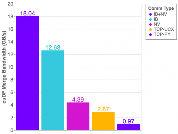
 Measured bandwidth of cuDF merge benchmark with UCX-Py on a DGX-1 server. Utilizing both InfiniBand and NVLink transports reaches just over 18 GB/s, InfiniBand without NVLink reaches 12.6 GB/s, NVLink with TCP achieves 4.3 GB/s, TCP over UCX throughput is of 2.8 GB/s and TCP with Python Sockets (meaning no UCX involved) only achieve 970 MB/s.
Figure 1: Measured bandwidth of cuDF merge benchmark with UCX-Py on a DGX-1 server.

Overall we see improvements using UCX-Py compared to using Python Sockets for TCP communication. However, there are some unexpected results. If NVLink is capable of 32GB/s and InfiniBand is 12GB/s, why then does InfiniBand perform better than NVLink? The answer is: topology! The layout of hardware interconnection is of great importance and can often be complex.
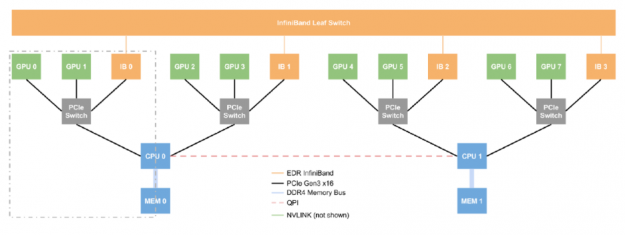
Represents the complex networking topology of a DGX-1 server
Figure 2: Networking topology of a DGX-1 server.

Figure 2 presents the layout of an NVIDIA DGX-1 server — we can think of this single box as a small supercomputer. The DGX-1 has eight P100 GPUs, four InfiniBand devices, and two CPUs. What is the most efficient route to take when passing data between GPU0 and GPU1? What about GPU2 and GPU7? GPU0 and GPU1 are connected via NVLink but GPU2 and GPU7 have direct communication lines, therefore, when passing data, we must perform two costly operations: Device-to-Host (moving data from GPU2 to the host) and Host-to-Device (moving data from the host to GPU7), and transferring data through main memory is expensive. Fortunately, a DGX-1 allows transfers between two GPUs that are not NVLink connected to use a more efficient transfer method than the costly operations described. With InfiniBand and GPUDirectRDMA, two GPUs can communicate without touching the main memory at all, allowing GPU7 to directly read GPU2’s memory via the InfiniBand interconnect only. 

Referring back to Figure 1, you can now see why only using InfiniBand outperforms the NVLink connection alone — Host-to-Device/Device-to-Host transfers are costly! However, when combining InfiniBand with NVLink we achieve more optimal performance. 

Further improvements

UCX-Py is under constant development, which means changes may occur without notice. Our ultimate commitment is to deliver high-performance communication to Python in a high-quality library package. With that said, we expect in the near future to keep on improving stability and ease-of-use, enabling users to benefit from enhanced performance with little to no effort to configure UCX-Py, thus automatically enabling accelerated communication hardware.

So far, we have tested UCX-Py mostly in DGX-1 and DGX-2 systems, where point-to-point and end-to-end performance was demonstrated. We scaled our testing up to one hundred Dask CUDA workers. We are constantly working to improve performance and stability, particularly for large scale workflows, and encourage users to engage with our team on GitHub and extend the discussion on UCX-Py.
Categories
Misc

Coming June to GFN Thursday: 38 More Games Streaming on GeForce NOW This Month

What a gamer wants. What a gamer needs. Games that’ll make you happy and cloud gaming that’ll set you free … to play your favorite PC games anywhere, anytime, on GeForce NOW. Get a sneak peek of all the exciting games coming in June this GFN Thursday. Starting with titles launching today. Keeping It Fresh Read article >

The post Coming June to GFN Thursday: 38 More Games Streaming on GeForce NOW This Month appeared first on The Official NVIDIA Blog.

Categories
Misc

NOOB: How to get TensorFlow model to run on Jetson Nano?

Hello –

I built a model (for ANPR) using TensorFlow and EasyOCR. Over the past week or so, getting TensorFlow to install on the Jetson Nano has been next to impossible. Tons of issues with it (some are documented) and overall I found one person that was able to get it running well which took over 50hrs to install on the Jetson Nano.

This said, there has to be a better way to get a TensorFlow model to run on a Jetson Nano. Does anyone know how to go about doing this? Is this where ONNX comes in (if so, any ideas/resources you might be able to point me to that shows how?)

Maybe I should go down another rabbit hole and try to do ANPR with PyTorch as I have read in the NVIDIA forums that PyTorch seems to be a bit easier to run on the Jetson line?

Any/all thoughts/help is much appreciated.

Thanks!

submitted by /u/InstantAmmo
[visit reddit] [comments]

Categories
Misc

Train Model for Pothole Detection to be used on raspberrypi

Hello, i followed random tutorials and tried training my custom model.

can somebody suggest me some tutorial or give me some tips on training an improved model?

any help would greatly be appreciated.

i am a beginner.

submitted by /u/abracadabra61
[visit reddit] [comments]

Categories
Misc

NVIDIA Spotlights GeForce Partners at COMPUTEX

Highlighting deep support from a flourishing roster of GeForce partners, NVIDIA’s Jeff Fisher delivered a virtual keynote at COMPUTEX 2021 in Taipei Tuesday. Fisher, senior vice president of NVIDIA’s GeForce business, announced a pair of powerful new gaming GPUs — the GeForce RTX 3080 Ti and GeForce RTX 3070 Ti — and detailed the fast-growing Read article >

The post NVIDIA Spotlights GeForce Partners at COMPUTEX appeared first on The Official NVIDIA Blog.

Categories
Misc

Multi-GPUs and custom training loops in TensorFlow 2

Multi-GPUs and custom training loops in TensorFlow 2 submitted by /u/ZnVjayBhY25l
[visit reddit] [comments]
Categories
Misc

NVIDIA Announces Upcoming Events for Financial Community

SANTA CLARA, Calif., June 01, 2021 (GLOBE NEWSWIRE) — NVIDIA will present at the following events for the financial community: Evercore ISI Inaugural TMT ConferenceMonday, June 7, at 10:15 …

Categories
Misc

DL server configuration for Unet training

My company is solving very specific task of semantic segmentation using small UNet and we need to speed up training. Our current workstation has single Tesla v100 and we are looking for new workstation with several A100 but can’t measure how much speed up we will get with the increase of GPU number with new Ampere architecture. The second question is do we need NVSwitch or NVLink for training UNet and what speed improvement it would give us. According to our budget we can possibly get DGX A100(40GB A100) or custom configuration without useless options for our task, for example NVSwitch. The only thing I find is NVidia Unet industrial performance but the evaluation has been done on DGX-1 and DGX A100 with NVLink/NVSwitch both so the impact of GPU interconnection is not obvious.

submitted by /u/gogasius
[visit reddit] [comments]

Categories
Misc

Why is it soooo slow to iterate over a specific dataset?

Situation:

I have a dataset (<class ‘tensorflow.python.data.ops.dataset_ops.MapDataset’>) which is a result of some neural network output. In order to get my final prediction, I am currently iterating over it as follows:

for row in dataset: ap_distance, an_distance = row y_pred.append(int(ap_distance.numpy() > an_distance.numpy())) 

The dataset has two columns, each holding a scalar wrapped in a tensor.

Problem:

The loop body is very simple, it takes < 1e-5 seconds to compute. Sadly, one iteration takes ca. 0.3 seconds, so fetching the next row from the dataset seems to take almost 0.3s! This behavior is very weird given my hardware (running on a rented GPU server with 16 AMD EPYC cores and 258GB RAM) and the fact that a colleague on his laptop can finish an iteration in 1-2 orders of magnitude less time than I can. The dataset has ca. 60k rows, hence it is unacceptable to wait for so long.

What I tried:

I tried mapping the above loop body onto every row of the dataset object, but sadly .numpy() is not available inside dataset.map()!

Questions:

  1. Why does it take so long to get a new row from the dataset?
  2. How can I fix this performance degradation?

submitted by /u/iMrFelix
[visit reddit] [comments]

Categories
Offsites

A Browsable Petascale Reconstruction of the Human Cortex

In January 2020 we released the fly “hemibrain” connectome — an online database providing the morphological structure and synaptic connectivity of roughly half of the brain of a fruit fly (Drosophila melanogaster). This database and its supporting visualization has reframed the way that neural circuits are studied and understood in the fly brain. While the fruit fly brain is small enough to attain a relatively complete map using modern mapping techniques, the insights gained are, at best, only partially informative to understanding the most interesting object in neuroscience — the human brain.

Today, in collaboration with the Lichtman laboratory at Harvard University, we are releasing the “H01” dataset, a 1.4 petabyte rendering of a small sample of human brain tissue, along with a companion paper, “A connectomic study of a petascale fragment of human cerebral cortex.” The H01 sample was imaged at 4nm-resolution by serial section electron microscopy, reconstructed and annotated by automated computational techniques, and analyzed for preliminary insights into the structure of the human cortex. The dataset comprises imaging data that covers roughly one cubic millimeter of brain tissue, and includes tens of thousands of reconstructed neurons, millions of neuron fragments, 130 million annotated synapses, 104 proofread cells, and many additional subcellular annotations and structures — all easily accessible with the Neuroglancer browser interface. H01 is thus far the largest sample of brain tissue imaged and reconstructed in this level of detail, in any species, and the first large-scale study of synaptic connectivity in the human cortex that spans multiple cell types across all layers of the cortex. The primary goals of this project are to produce a novel resource for studying the human brain and to improve and scale the underlying connectomics technologies.

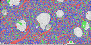
Petabyte connectomic reconstruction of a volume of human neocortex. Left: Small subvolume of the dataset. Right: A subgraph of 5000 neurons and excitatory (green) and inhibitory (red) connections in the dataset. The full graph (connectome) would be far too dense to visualize.

What is the Human Cortex?
The cerebral cortex is the thin surface layer of the brain found in vertebrate animals that has evolved most recently, showing the greatest variation in size among different mammals (it is especially large in humans). Each part of the cerebral cortex is six layered (e.g., L2), with different kinds of nerve cells (e.g., spiny stellate) in each layer. The cerebral cortex plays a crucial role in most higher level cognitive functions, such as thinking, memory, planning, perception, language, and attention. Although there has been some progress in understanding the macroscopic organization of this very complicated tissue, its organization at the level of individual nerve cells and their interconnecting synapses is largely unknown.

Human Brain Connectomics: From Surgical Biopsy to a 3D Database
Mapping the structure of the brain at the resolution of individual synapses requires high-resolution microscopy techniques that can image biochemically stabilized (fixed) tissue. We collaborated with brain surgeons at Massachusetts General Hospital in Boston (MGH) who sometimes remove pieces of normal human cerebral cortex when performing a surgery to cure epilepsy in order to gain access to a site in the deeper brain where an epileptic seizure is being initiated. Patients anonymously donated this tissue, which is normally discarded, to our colleagues in the Lichtman lab. The Harvard researchers cut the tissue into ~5300 individual 30 nanometer sections using an automated tape collecting ultra-microtome, mounted those sections onto silicon wafers, and then imaged the brain tissue at 4 nm resolution in a customized 61-beam parallelized scanning electron microscope for rapid image acquisition.

Imaging the ~5300 physical sections produced 225 million individual 2D images. Our team then computationally stitched and aligned this data to produce a single 3D volume. While the quality of the data was generally excellent, these alignment pipelines had to robustly handle a number of challenges, including imaging artifacts, missing sections, variation in microscope parameters, and physical stretching and compression of the tissue. Once aligned, a multiscale flood-filling network pipeline was applied (using thousands of Google Cloud TPUs) to produce a 3D segmentation of each individual cell in the tissue. Additional machine learning pipelines were applied to identify and characterize 130 million synapses, classify each 3D fragment into various “subcompartments” (e.g., axon, dendrite, or cell body), and identify other structures of interest such as myelin and cilia. Automated reconstruction results were imperfect, so manual efforts were used to “proofread” roughly one hundred cells in the data. Over time, we expect to add additional cells to this verified set through additional manual efforts and further advances in automation.

The H01 volume: roughly one cubic millimeter of human brain tissue captured in 1.4 petabytes of images.

The imaging data, reconstruction results, and annotations are viewable through an interactive web-based 3D visualization interface, called Neuroglancer, that was originally developed to visualize the fruit fly brain. Neuroglancer is available as open-source software, and widely used in the broader connectomics community. Several new features were introduced to support analysis of the H01 dataset, in particular support for searching for specific neurons in the dataset based on their type or other properties.

   
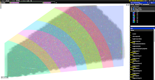
The volume spans all six cortical layers   Highlighting Layer 2 interneurons   Excitatory and inhibitory incoming synapses
   
Neuronal subcompartments classified   A Chandelier cell and some of the Pyramidal neurons it inhibits   Blood vessels traced throughout the volume
   
Serial contact between a pair of neurons   An axon with elaborate whorl structures   A neuron with unusual propensity for self-contact (Credit: Rachael Han)
The Neuroglancer interface to the H01 volume and annotations. The user can select specific cells on the basis of their layer and type, can view incoming and outgoing synapses for the cell, and much more. (Click on the images above to take you to the Neuroglancer view shown.)

Analysis of the Human Cortex
In a companion preprint, we show how H01 has already been used to study several interesting aspects of the organization of the human cortex. In particular, new cell types have been discovered, as well as the presence of “outlier” axonal inputs, which establish powerful synaptic connections with target dendrites. While these findings are a promising start, the vastness of the H01 dataset will provide a basis for many years of further study by researchers interested in the human cortex.

In order to accelerate the analysis of H01, we also provide embeddings of the H01 data that were generated by a neural network trained using a variant of the SimCLR self-supervised learning technique. These embeddings provide highly informative representations of local parts of the dataset that can be used to rapidly annotate new structures and develop new ways of clustering and categorizing brain structures according to purely data-driven criteria. We trained these embeddings using Google Cloud TPU pods and then performed inference at roughly four billion data locations spread throughout the volume.

Managing Dataset Size with Improved Compression
H01 is a petabyte-scale dataset, but is only one-millionth the volume of an entire human brain. Serious technical challenges remain in scaling up synapse-level brain mapping to an entire mouse brain (500x bigger than H01), let alone an entire human brain. One of these challenges is data storage: a mouse brain could generate an exabyte worth of data, which is costly to store. To address this, we are today also releasing a paper, “Denoising-based Image Compression for Connectomics”, that details how a machine learning-based denoising strategy can be used to compress data, such as H01, at least 17-fold (dashed line in the figure below), with negligible loss of accuracy in the automated reconstruction.

Reconstruction quality of noisy and denoised images as a function of compression rate for JPEG XL (JXL) and AV Image Format (AVIF) codecs. Points and lines show the means, and the shaded area covers ±1 standard deviation around the mean.

Random variations in the electron microscopy imaging process lead to image noise that is difficult to compress even in principle, as the noise lacks spatial correlations or other structure that could be described with fewer bytes. Therefore we acquired images of the same piece of tissue in both a “fast” acquisition regime (resulting in high amounts of noise) and a “slow” acquisition regime (resulting in low amounts of noise) and then trained a neural network to infer “slow” scans from “fast” scans. Standard image compression codecs were then able to (lossily) compress the “virtual” slow scans with fewer artifacts compared to the raw data. We believe this advance has the potential to significantly mitigate the costs associated with future large scale connectomics projects.

Next Steps
But storage is not the only problem. The sheer size of future data sets will require developing new strategies for researchers to organize and access the rich information inherent in connectomic data. These are challenges that will require new modes of interaction between humans and the brain mapping data that will be forthcoming.