We pick up where the first post in this series left us: confronting the task of multi-step time-series forecasting.
Our first attempt was a workaround of sorts. The model had been trained to deliver a single prediction, corresponding to the very next point in time. Thus, if we needed a longer forecast, all we could do is use that prediction and feed it back to the model, moving the input sequence by one value (from ([x_{t-n}, …, x_t]) to ([x_{t-n-1}, …, x_{t+1}]), say).
In contrast, the new model will be designed – and trained – to forecast a configurable number of observations at once. The architecture will still be basic – about as basic as possible, given the task – and thus, can serve as a baseline for later attempts.
Data input
We work with the same data as before, vic_elec from tsibbledata.
Compared to last time though, the dataset class has to change. While, previously, for each batch item the target (y) was a single value, it now is a vector, just like the input, x. And just like n_timesteps was (and still is) used to specify the length of the input sequence, there is now a second parameter, n_forecast, to configure target size.
In our example, n_timesteps and n_forecast are set to the same value, but there is no need for this to be the case. You could equally well train on week-long sequences and then forecast developments over a single day, or a month.
Apart from the fact that .getitem() now returns a vector for y as well as x, there is not much to be said about dataset creation. Here is the complete code to set up the data input pipeline:
n_timesteps <- 7 * 24 * 2
n_forecast <- 7 * 24 * 2
batch_size <- 32

vic_elec_get_year <- function(year, month = NULL) {
  vic_elec %>%
    filter(year(Date) == year, month(Date) == if (is.null(month)) month(Date) else month) %>%
    as_tibble() %>%
    select(Demand)
}

elec_train <- vic_elec_get_year(2012) %>% as.matrix()
elec_valid <- vic_elec_get_year(2013) %>% as.matrix()
elec_test <- vic_elec_get_year(2014, 1) %>% as.matrix()

train_mean <- mean(elec_train)
train_sd <- sd(elec_train)

elec_dataset <- dataset(
  name = "elec_dataset",

  initialize = function(x, n_timesteps, n_forecast, sample_frac = 1) {

    self$n_timesteps <- n_timesteps
    self$n_forecast <- n_forecast
    self$x <- torch_tensor((x - train_mean) / train_sd)

    n <- length(self$x) - self$n_timesteps - self$n_forecast + 1

    self$starts <- sort(sample.int(
      n = n,
      size = n * sample_frac
    ))

  },

  .getitem = function(i) {

    start <- self$starts[i]
    end <- start + self$n_timesteps - 1
    pred_length <- self$n_forecast

    list(
      x = self$x[start:end],
      y = self$x[(end + 1):(end + pred_length)]$squeeze(2)
    )

  },

  .length = function() {
    length(self$starts)
  }
)

train_ds <- elec_dataset(elec_train, n_timesteps, n_forecast, sample_frac = 0.5)
train_dl <- train_ds %>% dataloader(batch_size = batch_size, shuffle = TRUE)

valid_ds <- elec_dataset(elec_valid, n_timesteps, n_forecast, sample_frac = 0.5)
valid_dl <- valid_ds %>% dataloader(batch_size = batch_size)

test_ds <- elec_dataset(elec_test, n_timesteps, n_forecast)
test_dl <- test_ds %>% dataloader(batch_size = 1)
Model
The model replaces the single linear layer that, in the previous post, had been tasked with outputting the final prediction, with a small network, complete with two linear layers and – optional – dropout.
In forward(), we first apply the RNN, and just like in the previous post, we make use of the outputs only; or more specifically, the output corresponding to the final time step. (See that previous post for a detailed discussion of what a torch RNN returns.)
model <- nn_module(

  initialize = function(type, input_size, hidden_size, linear_size, output_size,
                        num_layers = 1, dropout = 0, linear_dropout = 0) {

    self$type <- type
    self$num_layers <- num_layers
    self$linear_dropout <- linear_dropout

    self$rnn <- if (self$type == "gru") {
      nn_gru(
        input_size = input_size,
        hidden_size = hidden_size,
        num_layers = num_layers,
        dropout = dropout,
        batch_first = TRUE
      )
    } else {
      nn_lstm(
        input_size = input_size,
        hidden_size = hidden_size,
        num_layers = num_layers,
        dropout = dropout,
        batch_first = TRUE
      )
    }

    self$mlp <- nn_sequential(
      nn_linear(hidden_size, linear_size),
      nn_relu(),
      nn_dropout(linear_dropout),
      nn_linear(linear_size, output_size)
    )

  },

  forward = function(x) {

    x <- self$rnn(x)
    x[[1]][ ,-1, ..] %>%
      self$mlp()

  }

)
For model instantiation, we now have an additional configuration parameter, related to the amount of dropout between the two linear layers.
net <- model(
  "gru", input_size = 1, hidden_size = 32, linear_size = 512, output_size = n_forecast, linear_dropout = 0
  )

# training RNNs on the GPU currently prints a warning that may clutter
# the console
# see https://github.com/mlverse/torch/issues/461
# alternatively, use
# device <- "cpu"
device <- torch_device(if (cuda_is_available()) "cuda" else "cpu")

net <- net$to(device = device)
Training
The training procedure is completely unchanged.
optimizer <- optim_adam(net$parameters, lr = 0.001)

num_epochs <- 30

train_batch <- function(b) {

  optimizer$zero_grad()
  output <- net(b$x$to(device = device))
  target <- b$y$to(device = device)

  loss <- nnf_mse_loss(output, target)
  loss$backward()
  optimizer$step()

  loss$item()
}

valid_batch <- function(b) {

  output <- net(b$x$to(device = device))
  target <- b$y$to(device = device)

  loss <- nnf_mse_loss(output, target)
  loss$item()

}

for (epoch in 1:num_epochs) {

  net$train()
  train_loss <- c()

  coro::loop(for (b in train_dl) {
    loss <-train_batch(b)
    train_loss <- c(train_loss, loss)
  })

  cat(sprintf("nEpoch %d, training: loss: %3.5f n", epoch, mean(train_loss)))

  net$eval()
  valid_loss <- c()

  coro::loop(for (b in valid_dl) {
    loss <- valid_batch(b)
    valid_loss <- c(valid_loss, loss)
  })

  cat(sprintf("nEpoch %d, validation: loss: %3.5f n", epoch, mean(valid_loss)))
}
# Epoch 1, training: loss: 0.65737
#
# Epoch 1, validation: loss: 0.54586
#
# Epoch 2, training: loss: 0.43991
#
# Epoch 2, validation: loss: 0.50588
#
# Epoch 3, training: loss: 0.42161
#
# Epoch 3, validation: loss: 0.50031
#
# Epoch 4, training: loss: 0.41718
#
# Epoch 4, validation: loss: 0.48703
#
# Epoch 5, training: loss: 0.39498
#
# Epoch 5, validation: loss: 0.49572
#
# Epoch 6, training: loss: 0.38073
#
# Epoch 6, validation: loss: 0.46813
#
# Epoch 7, training: loss: 0.36472
#
# Epoch 7, validation: loss: 0.44957
#
# Epoch 8, training: loss: 0.35058
#
# Epoch 8, validation: loss: 0.44440
#
# Epoch 9, training: loss: 0.33880
#
# Epoch 9, validation: loss: 0.41995
#
# Epoch 10, training: loss: 0.32545
#
# Epoch 10, validation: loss: 0.42021
#
# Epoch 11, training: loss: 0.31347
#
# Epoch 11, validation: loss: 0.39514
#
# Epoch 12, training: loss: 0.29622
#
# Epoch 12, validation: loss: 0.38146
#
# Epoch 13, training: loss: 0.28006
#
# Epoch 13, validation: loss: 0.37754
#
# Epoch 14, training: loss: 0.27001
#
# Epoch 14, validation: loss: 0.36636
#
# Epoch 15, training: loss: 0.26191
#
# Epoch 15, validation: loss: 0.35338
#
# Epoch 16, training: loss: 0.25533
#
# Epoch 16, validation: loss: 0.35453
#
# Epoch 17, training: loss: 0.25085
#
# Epoch 17, validation: loss: 0.34521
#
# Epoch 18, training: loss: 0.24686
#
# Epoch 18, validation: loss: 0.35094
#
# Epoch 19, training: loss: 0.24159
#
# Epoch 19, validation: loss: 0.33776
#
# Epoch 20, training: loss: 0.23680
#
# Epoch 20, validation: loss: 0.33974
#
# Epoch 21, training: loss: 0.23070
#
# Epoch 21, validation: loss: 0.34069
#
# Epoch 22, training: loss: 0.22761
#
# Epoch 22, validation: loss: 0.33724
#
# Epoch 23, training: loss: 0.22390
#
# Epoch 23, validation: loss: 0.34013
#
# Epoch 24, training: loss: 0.22155
#
# Epoch 24, validation: loss: 0.33460
#
# Epoch 25, training: loss: 0.21820
#
# Epoch 25, validation: loss: 0.33755
#
# Epoch 26, training: loss: 0.22134
#
# Epoch 26, validation: loss: 0.33678
#
# Epoch 27, training: loss: 0.21061
#
# Epoch 27, validation: loss: 0.33108
#
# Epoch 28, training: loss: 0.20496
#
# Epoch 28, validation: loss: 0.32769
#
# Epoch 29, training: loss: 0.20223
#
# Epoch 29, validation: loss: 0.32969
#
# Epoch 30, training: loss: 0.20022
#
# Epoch 30, validation: loss: 0.33331
From the way loss decreases on the training set, we conclude that, yes, the model is learning something. It probably would continue improving for quite some epochs still. We do, however, see less of an improvement on the validation set.
Naturally, now we’re curious about test-set predictions. (Remember, for testing we’re choosing the “particularly hard” month of January, 2014 – particularly hard because of a heatwave that resulted in exceptionally high demand.)
Evaluation
With no loop to be coded, evaluation now becomes pretty straightforward:
net$eval()

test_preds <- vector(mode = "list", length = length(test_dl))

i <- 1

coro::loop(for (b in test_dl) {

  input <- b$x
  output <- net(input$to(device = device))
  preds <- as.numeric(output)

  test_preds[[i]] <- preds
  i <<- i + 1

})

vic_elec_jan_2014 <- vic_elec %>%
  filter(year(Date) == 2014, month(Date) == 1)

test_pred1 <- test_preds[[1]]
test_pred1 <- c(rep(NA, n_timesteps), test_pred1, rep(NA, nrow(vic_elec_jan_2014) - n_timesteps - n_forecast))

test_pred2 <- test_preds[[408]]
test_pred2 <- c(rep(NA, n_timesteps + 407), test_pred2, rep(NA, nrow(vic_elec_jan_2014) - 407 - n_timesteps - n_forecast))

test_pred3 <- test_preds[[817]]
test_pred3 <- c(rep(NA, nrow(vic_elec_jan_2014) - n_forecast), test_pred3)


preds_ts <- vic_elec_jan_2014 %>%
  select(Demand) %>%
  add_column(
    mlp_ex_1 = test_pred1 * train_sd + train_mean,
    mlp_ex_2 = test_pred2 * train_sd + train_mean,
    mlp_ex_3 = test_pred3 * train_sd + train_mean) %>%
  pivot_longer(-Time) %>%
  update_tsibble(key = name)


preds_ts %>%
  autoplot() +
  scale_colour_manual(values = c("#08c5d1", "#00353f", "#ffbf66", "#d46f4d")) +
  theme_minimal()

(#fig:unnamed-chunk-6)One-week-ahead predictions for January, 2014.
Compare this to the forecast obtained by feeding back predictions. The demand profiles over the day look a lot more realistic now. How about the phases of extreme demand? Evidently, these are not reflected in the forecast, not any more than in the “loop technique”. In fact, the forecast allows for interesting insights into this model’s personality: Apparently, it really likes fluctuating around the mean – “prime” it with inputs that oscillate around a significantly higher level, and it will quickly shift back to its comfort zone.
Discussion
Seeing how, above, we provided an option to use dropout inside the MLP, you may be wondering if this would help with forecasts on the test set. Turns out it did not, in my experiments. Maybe this is not so strange either: How, absent external cues (temperature), should the network know that high demand is coming up?
In our analysis, we can make an additional distinction. With the first week of predictions, what we see is a failure to anticipate something that could not reasonably have been anticipated (two, or two-and-a-half, say, days of exceptionally high demand). In the second, all the network would have had to do was stay at the current, elevated level. It will be interesting to see how this is handled by the architectures we discuss next.
Finally, an additional idea you may have had is – what if we used temperature as a second input variable? As a matter of fact, training performance indeed improved, but no performance impact was observed on the validation and test sets. Still, you may find the code useful – it is easily extended to datasets with more predictors. Therefore, we reproduce it in the appendix.
Thanks for reading!
Appendix
# Data input code modified to accommodate two predictors

n_timesteps <- 7 * 24 * 2
n_forecast <- 7 * 24 * 2

vic_elec_get_year <- function(year, month = NULL) {
  vic_elec %>%
    filter(year(Date) == year, month(Date) == if (is.null(month)) month(Date) else month) %>%
    as_tibble() %>%
    select(Demand, Temperature)
}

elec_train <- vic_elec_get_year(2012) %>% as.matrix()
elec_valid <- vic_elec_get_year(2013) %>% as.matrix()
elec_test <- vic_elec_get_year(2014, 1) %>% as.matrix()

train_mean_demand <- mean(elec_train[ , 1])
train_sd_demand <- sd(elec_train[ , 1])

train_mean_temp <- mean(elec_train[ , 2])
train_sd_temp <- sd(elec_train[ , 2])

elec_dataset <- dataset(
  name = "elec_dataset",

  initialize = function(data, n_timesteps, n_forecast, sample_frac = 1) {

    demand <- (data[ , 1] - train_mean_demand) / train_sd_demand
    temp <- (data[ , 2] - train_mean_temp) / train_sd_temp
    self$x <- cbind(demand, temp) %>% torch_tensor()

    self$n_timesteps <- n_timesteps
    self$n_forecast <- n_forecast

    n <- nrow(self$x) - self$n_timesteps - self$n_forecast + 1
    self$starts <- sort(sample.int(
      n = n,
      size = n * sample_frac
    ))

  },

  .getitem = function(i) {

    start <- self$starts[i]
    end <- start + self$n_timesteps - 1
    pred_length <- self$n_forecast

    list(
      x = self$x[start:end, ],
      y = self$x[(end + 1):(end + pred_length), 1]
    )

  },

  .length = function() {
    length(self$starts)
  }

)

### rest identical to single-predictor code above
Photo by Monica Bourgeau on Unsplash
 The focus of this post is on using commercial off-the-shelf (COTS) hardware running BIG-IP VE with NVIDIA NICs and switches to achieve 100G+ throughput in an ultra-high, high-density solution that is available today.
  With this latest .4 release, NVIDIA Merlin delivers a new API and inference support that helps streamline the recommender workflow.
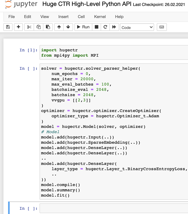
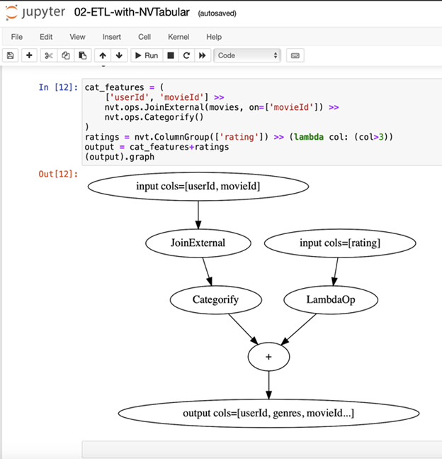
 Through the tutorial, you will create a QA service with Bidirectional Encoder Representations from Transformers (BERT).
 Telcos require fast, time-synchronized, precise, affordable, and secure networking for 5G rollouts. The key to this is a solution that offers high programmability, scalability, and performance combined with intelligent accelerators and offloads with low-latency and fast packet processing capabilities and GPU acceleration at the edge.
 NVTX is a C-based Application Programming Interface (API) for annotating events, code ranges, and resources in your applications.
 The new launcher provides the latest news and updates about Omniverse, as well as the exchange where users can install and update applications and components like Omniverse Create, Kit, Cache, Drive and the Autodesk Maya Connector.
 Kit. The Scene Description and in-memory model is based on Pixar’s USD. Omniverse Create takes advantage of the advanced workflows of USD like Layers, Variants, Instancing and more.