Brain image segmentation with torch

When what is not enough

True, sometimes it’s vital to distinguish between different
kinds of objects. Is that a car speeding towards me, in which case
I’d better jump out of the way? Or is it a huge Doberman (in
which case I’d probably do the same)? Often in real life though,
instead of coarse-grained classification, what is needed is
fine-grained segmentation.

Zooming in on images, we’re not looking for a single label;
instead, we want to classify every pixel according to some
criterion:

• In medicine, we may want to distinguish between different cell
  types, or identify tumors.

• In various earth sciences, satellite data are used to segment
  terrestrial surfaces.

• To enable use of custom backgrounds, video-conferencing software
  has to be able to tell foreground from background.

Image segmentation is a form of supervised learning: Some kind
of ground truth is needed. Here, it comes in form of a mask – an
image, of spatial resolution identical to that of the input data,
that designates the true class for every pixel. Accordingly,
classification loss is calculated pixel-wise; losses are then
summed up to yield an aggregate to be used in optimization.

The “canonical” architecture for image segmentation is U-Net
(around since 2015).

U-Net

Here is the prototypical U-Net, as depicted in the original
Rönneberger et al.paper (Ronneberger, Fischer, and Brox
2015).

Of this architecture, numerous variants exist. You could use
different layer sizes, activations, ways to achieve downsizing and
upsizing, and more. However, there is one defining characteristic:
the U-shape, stabilized by the “bridges” crossing over
horizontally at all levels.

In a nutshell, the left-hand side of the U resembles the
convolutional architectures used in image classification. It
successively reduces spatial resolution. At the same time, another
dimension – the channels dimension – is used to build up a
hierarchy of features, ranging from very basic to very
specialized.

Unlike in classification, however, the output should have the
same spatial resolution as the input. Thus, we need to upsize again
– this is taken care of by the right-hand side of the U. But, how
are we going to arrive at a good per-pixel classification, now that
so much spatial information has been lost?

This is what the “bridges” are for: At each level, the input
to an upsampling layer is a concatenation of the previous layer’s
output – which went through the whole compression/decompression
routine – and some preserved intermediate representation from the
downsizing phase. In this way, a U-Net architecture combines
attention to detail with feature extraction.

Brain image segmentation

With U-Net, domain applicability is as broad as the architecture
is flexible. Here, we want to detect abnormalities in brain scans.
The dataset, used in Buda, Saha, and Mazurowski (2019), contains
MRI images together with manually created
FLAIR abnormality segmentation masks. It is available on
Kaggle.

Nicely, the paper is accompanied by a GitHub
repository. Below, we closely follow (though not exactly
replicate) the authors’ preprocessing and data augmentation
code.

As is often the case in medical imaging, there is notable class
imbalance in the data. For every patient, sections have been taken
at multiple positions. (Number of sections per patient varies.)
Most sections do not exhibit any lesions; the corresponding masks
are colored black everywhere.

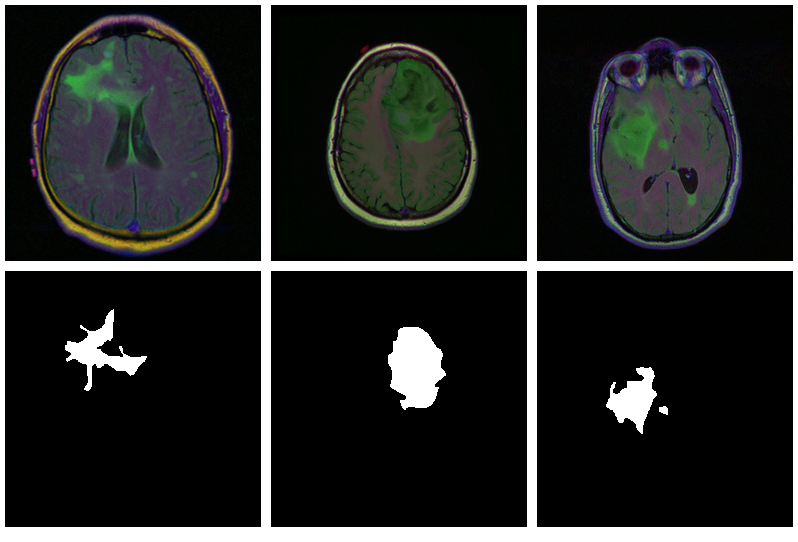
Here are three examples where the masks do indicate
abnormalities:

Let’s see if we can build a U-Net that generates such masks
for us.

Data

Before you start typing, here is a
Colaboratory notebook to conveniently follow along.

We use pins to obtain the data. Please see this
introduction if you haven’t used that package before.

# deep learning (incl. dependencies) library(torch) library(torchvision) # data wrangling library(tidyverse) library(zeallot) # image processing and visualization library(magick) library(cowplot) # dataset loading library(pins) library(zip) torch_manual_seed(777) set.seed(777) # use your own kaggle.json here pins::board_register_kaggle(token = "~/kaggle.json") files <- pins::pin_get("mateuszbuda/lgg-mri-segmentation", board = "kaggle", extract = FALSE)

The dataset is not that big – it includes scans from 110
different patients – so we’ll have to do with just a training
and a validation set. (Don’t do this in real life, as you’ll
inevitably end up fine-tuning on the latter.)

train_dir <- "data/mri_train" valid_dir <- "data/mri_valid" if(dir.exists(train_dir)) unlink(train_dir, recursive = TRUE, force = TRUE) if(dir.exists(valid_dir)) unlink(valid_dir, recursive = TRUE, force = TRUE) zip::unzip(files, exdir = "data") file.rename("data/kaggle_3m", train_dir) # this is a duplicate, again containing kaggle_3m (evidently a packaging error on Kaggle) # we just remove it unlink("data/lgg-mri-segmentation", recursive = TRUE) dir.create(valid_dir)

Of those 110 patients, we keep 30 for validation. Some more file
manipulations, and we’re set up with a nice hierarchical
structure, with train_dir and valid_dir holding their per-patient
sub-directories, respectively.

valid_indices <- sample(1:length(patients), 30) patients <- list.dirs(train_dir, recursive = FALSE) for (i in valid_indices) { dir.create(file.path(valid_dir, basename(patients[i]))) for (f in list.files(patients[i])) { file.rename(file.path(train_dir, basename(patients[i]), f), file.path(valid_dir, basename(patients[i]), f)) } unlink(file.path(train_dir, basename(patients[i])), recursive = TRUE) }

We now need a dataset that knows what to do with these
files.

Dataset

Like every torch dataset, this one has initialize() and
.getitem() methods. initialize() creates an inventory of scan and
mask file names, to be used by .getitem() when it actually reads
those files. In contrast to what we’ve seen in previous posts,
though , .getitem() does not simply return input-target pairs in
order. Instead, whenever the parameter random_sampling is true, it
will perform weighted sampling, preferring items with sizable
lesions. This option will be used for the training set, to counter
the class imbalance mentioned above.

The other way training and validation sets will differ is use of
data augmentation. Training images/masks may be flipped, re-sized,
and rotated; probabilities and amounts are configurable.

An instance of brainseg_dataset encapsulates all this
functionality:

brainseg_dataset <- dataset( name = "brainseg_dataset", initialize = function(img_dir, augmentation_params = NULL, random_sampling = FALSE) { self$images <- tibble( img = grep( list.files( img_dir, full.names = TRUE, pattern = "tif", recursive = TRUE ), pattern = 'mask', invert = TRUE, value = TRUE ), mask = grep( list.files( img_dir, full.names = TRUE, pattern = "tif", recursive = TRUE ), pattern = 'mask', value = TRUE ) ) self$slice_weights <- self$calc_slice_weights(self$images$mask) self$augmentation_params <- augmentation_params self$random_sampling <- random_sampling }, .getitem = function(i) { index <- if (self$random_sampling == TRUE) sample(1:self$.length(), 1, prob = self$slice_weights) else i img <- self$images$img[index] %>% image_read() %>% transform_to_tensor() mask <- self$images$mask[index] %>% image_read() %>% transform_to_tensor() %>% transform_rgb_to_grayscale() %>% torch_unsqueeze(1) img <- self$min_max_scale(img) if (!is.null(self$augmentation_params)) { scale_param <- self$augmentation_params[1] c(img, mask) %<-% self$resize(img, mask, scale_param) rot_param <- self$augmentation_params[2] c(img, mask) %<-% self$rotate(img, mask, rot_param) flip_param <- self$augmentation_params[3] c(img, mask) %<-% self$flip(img, mask, flip_param) } list(img = img, mask = mask) }, .length = function() { nrow(self$images) }, calc_slice_weights = function(masks) { weights <- map_dbl(masks, function(m) { img <- as.integer(magick::image_data(image_read(m), channels = "gray")) sum(img / 255) }) sum_weights <- sum(weights) num_weights <- length(weights) weights <- weights %>% map_dbl(function(w) { w <- (w + sum_weights * 0.1 / num_weights) / (sum_weights * 1.1) }) weights }, min_max_scale = function(x) { min = x$min()$item() max = x$max()$item() x$clamp_(min = min, max = max) x$add_(-min)$div_(max - min + 1e-5) x }, resize = function(img, mask, scale_param) { img_size <- dim(img)[2] rnd_scale <- runif(1, 1 - scale_param, 1 + scale_param) img <- transform_resize(img, size = rnd_scale * img_size) mask <- transform_resize(mask, size = rnd_scale * img_size) diff <- dim(img)[2] - img_size if (diff > 0) { top <- ceiling(diff / 2) left <- ceiling(diff / 2) img <- transform_crop(img, top, left, img_size, img_size) mask <- transform_crop(mask, top, left, img_size, img_size) } else { img <- transform_pad(img, padding = -c( ceiling(diff / 2), floor(diff / 2), ceiling(diff / 2), floor(diff / 2) )) mask <- transform_pad(mask, padding = -c( ceiling(diff / 2), floor(diff / 2), ceiling(diff / 2), floor(diff / 2) )) } list(img, mask) }, rotate = function(img, mask, rot_param) { rnd_rot <- runif(1, 1 - rot_param, 1 + rot_param) img <- transform_rotate(img, angle = rnd_rot) mask <- transform_rotate(mask, angle = rnd_rot) list(img, mask) }, flip = function(img, mask, flip_param) { rnd_flip <- runif(1) if (rnd_flip > flip_param) { img <- transform_hflip(img) mask <- transform_hflip(mask) } list(img, mask) } )

After instantiation, we see we have 2977 training pairs and 952
validation pairs, respectively:

train_ds <- brainseg_dataset( train_dir, augmentation_params = c(0.05, 15, 0.5), random_sampling = TRUE ) length(train_ds) # 2977 valid_ds <- brainseg_dataset( valid_dir, augmentation_params = NULL, random_sampling = FALSE ) length(valid_ds) # 952

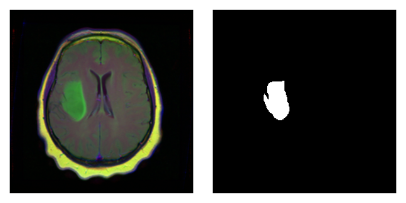
As a correctness check, let’s plot an image and associated
mask:

par(mfrow = c(1, 2), mar = c(0, 1, 0, 1)) img_and_mask <- valid_ds[27] img <- img_and_mask[[1]] mask <- img_and_mask[[2]] img$permute(c(2, 3, 1)) %>% as.array() %>% as.raster() %>% plot() mask$squeeze() %>% as.array() %>% as.raster() %>% plot()

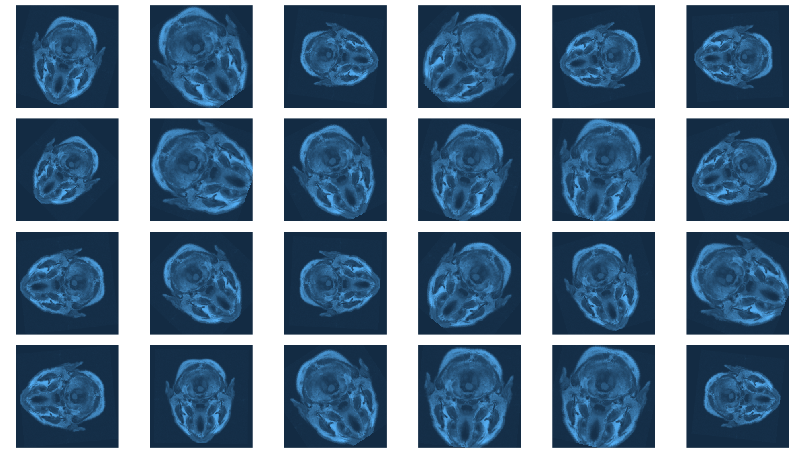
With torch, it is straightforward to inspect what happens when
you change augmentation-related parameters. We just pick a pair
from the validation set, which has not had any augmentation applied
as yet, and call valid_ds$<augmentation_func()> directly.
Just for fun, let’s use more “extreme” parameters here than
we do in actual training. (Actual training uses the settings from
Mateusz’ GitHub repository, which we assume have been carefully
chosen for optimal performance.1)

img_and_mask <- valid_ds[77] img <- img_and_mask[[1]] mask <- img_and_mask[[2]] imgs <- map (1:24, function(i) { # scale factor; train_ds really uses 0.05 c(img, mask) %<-% valid_ds$resize(img, mask, 0.2) c(img, mask) %<-% valid_ds$flip(img, mask, 0.5) # rotation angle; train_ds really uses 15 c(img, mask) %<-% valid_ds$rotate(img, mask, 90) img %>% transform_rgb_to_grayscale() %>% as.array() %>% as_tibble() %>% rowid_to_column(var = "Y") %>% gather(key = "X", value = "value", -Y) %>% mutate(X = as.numeric(gsub("V", "", X))) %>% ggplot(aes(X, Y, fill = value)) + geom_raster() + theme_void() + theme(legend.position = "none") + theme(aspect.ratio = 1) }) plot_grid(plotlist = imgs, nrow = 4)

Now we still need the data loaders, and then, nothing keeps us
from proceeding to the next big task: building the model.

batch_size <- 4 train_dl <- dataloader(train_ds, batch_size) valid_dl <- dataloader(valid_ds, batch_size)

Model

Our model nicely illustrates the kind of modular code that comes
“naturally” with torch. We approach things top-down, starting
with the U-Net container itself.

unet takes care of the global composition – how far “down”
do we go, shrinking the image while incrementing the number of
filters, and then how do we go “up” again?

Importantly, it is also in the system’s memory. In forward(),
it keeps track of layer outputs seen going “down”, to be added
back in going “up”.

unet <- nn_module( "unet", initialize = function(channels_in = 3, n_classes = 1, depth = 5, n_filters = 6) { self$down_path <- nn_module_list() prev_channels <- channels_in for (i in 1:depth) { self$down_path$append(down_block(prev_channels, 2 ^ (n_filters + i - 1))) prev_channels <- 2 ^ (n_filters + i -1) } self$up_path <- nn_module_list() for (i in ((depth - 1):1)) { self$up_path$append(up_block(prev_channels, 2 ^ (n_filters + i - 1))) prev_channels <- 2 ^ (n_filters + i - 1) } self$last = nn_conv2d(prev_channels, n_classes, kernel_size = 1) }, forward = function(x) { blocks <- list() for (i in 1:length(self$down_path)) { x <- self$down_path[[i]](x) if (i != length(self$down_path)) { blocks <- c(blocks, x) x <- nnf_max_pool2d(x, 2) } } for (i in 1:length(self$up_path)) { x <- self$up_path[[i]](x, blocks[[length(blocks) - i + 1]]$to(device = device)) } torch_sigmoid(self$last(x)) } )

unet delegates to two containers just below it in the hierarchy:
down_block and up_block. While down_block is “just” there for
aesthetic reasons (it immediately delegates to its own workhorse,
conv_block), in up_block we see the U-Net “bridges” in
action.

down_block <- nn_module( "down_block", initialize = function(in_size, out_size) { self$conv_block <- conv_block(in_size, out_size) }, forward = function(x) { self$conv_block(x) } ) up_block <- nn_module( "up_block", initialize = function(in_size, out_size) { self$up = nn_conv_transpose2d(in_size, out_size, kernel_size = 2, stride = 2) self$conv_block = conv_block(in_size, out_size) }, forward = function(x, bridge) { up <- self$up(x) torch_cat(list(up, bridge), 2) %>% self$conv_block() } )

Finally, a conv_block is a sequential structure containing
convolutional, ReLU, and dropout layers.

conv_block <- nn_module( "conv_block", initialize = function(in_size, out_size) { self$conv_block <- nn_sequential( nn_conv2d(in_size, out_size, kernel_size = 3, padding = 1), nn_relu(), nn_dropout(0.6), nn_conv2d(out_size, out_size, kernel_size = 3, padding = 1), nn_relu() ) }, forward = function(x){ self$conv_block(x) } )

Now instantiate the model, and possibly, move it to the GPU:

device <- torch_device(if(cuda_is_available()) "cuda" else "cpu") model <- unet(depth = 5)$to(device = device)

Optimization

We train our model with a combination of cross entropy and

dice loss.

The latter, though not shipped with torch, may be implemented
manually:

calc_dice_loss <- function(y_pred, y_true) { smooth <- 1 y_pred <- y_pred$view(-1) y_true <- y_true$view(-1) intersection <- (y_pred * y_true)$sum() 1 - ((2 * intersection + smooth) / (y_pred$sum() + y_true$sum() + smooth)) } dice_weight <- 0.3

Optimization uses stochastic gradient descent (SGD), together
with the one-cycle learning rate scheduler introduced in the
context of
image classification with torch.

optimizer <- optim_sgd(model$parameters, lr = 0.1, momentum = 0.9) num_epochs <- 20 scheduler <- lr_one_cycle( optimizer, max_lr = 0.1, steps_per_epoch = length(train_dl), epochs = num_epochs )

Training

The training loop then follows the usual scheme. One thing to
note: Every epoch, we save the model (using torch_save()), so we
can later pick the best one, should performance have degraded
thereafter.

train_batch <- function(b) { optimizer$zero_grad() output <- model(b[[1]]$to(device = device)) target <- b[[2]]$to(device = device) bce_loss <- nnf_binary_cross_entropy(output, target) dice_loss <- calc_dice_loss(output, target) loss <- dice_weight * dice_loss + (1 - dice_weight) * bce_loss loss$backward() optimizer$step() scheduler$step() list(bce_loss$item(), dice_loss$item(), loss$item()) } valid_batch <- function(b) { output <- model(b[[1]]$to(device = device)) target <- b[[2]]$to(device = device) bce_loss <- nnf_binary_cross_entropy(output, target) dice_loss <- calc_dice_loss(output, target) loss <- dice_weight * dice_loss + (1 - dice_weight) * bce_loss list(bce_loss$item(), dice_loss$item(), loss$item()) } for (epoch in 1:num_epochs) { model$train() train_bce <- c() train_dice <- c() train_loss <- c() for (b in enumerate(train_dl)) { c(bce_loss, dice_loss, loss) %<-% train_batch(b) train_bce <- c(train_bce, bce_loss) train_dice <- c(train_dice, dice_loss) train_loss <- c(train_loss, loss) } torch_save(model, paste0("model_", epoch, ".pt")) cat(sprintf("nEpoch %d, training: loss:%3f, bce: %3f, dice: %3fn", epoch, mean(train_loss), mean(train_bce), mean(train_dice))) model$eval() valid_bce <- c() valid_dice <- c() valid_loss <- c() i <- 0 for (b in enumerate(valid_dl)) { i <<- i + 1 c(bce_loss, dice_loss, loss) %<-% valid_batch(b) valid_bce <- c(valid_bce, bce_loss) valid_dice <- c(valid_dice, dice_loss) valid_loss <- c(valid_loss, loss) } cat(sprintf("nEpoch %d, validation: loss:%3f, bce: %3f, dice: %3fn", epoch, mean(valid_loss), mean(valid_bce), mean(valid_dice))) }

Epoch 1, training: loss:0.304232, bce: 0.148578, dice: 0.667423 Epoch 1, validation: loss:0.333961, bce: 0.127171, dice: 0.816471 Epoch 2, training: loss:0.194665, bce: 0.101973, dice: 0.410945 Epoch 2, validation: loss:0.341121, bce: 0.117465, dice: 0.862983 [...] Epoch 19, training: loss:0.073863, bce: 0.038559, dice: 0.156236 Epoch 19, validation: loss:0.302878, bce: 0.109721, dice: 0.753577 Epoch 20, training: loss:0.070621, bce: 0.036578, dice: 0.150055 Epoch 20, validation: loss:0.295852, bce: 0.101750, dice: 0.748757

Evaluation

In this run, it is the final model that performs best on the
validation set. Still, we’d like to show how to load a saved
model, using torch_load() .

Once loaded, put the model into eval mode:

saved_model <- torch_load("model_20.pt") model <- saved_model model$eval()

Now, since we don’t have a separate test set, we already know
the average out-of-sample metrics; but in the end, what we care
about are the generated masks. Let’s view some, displaying ground
truth and MRI scans for comparison.

# without random sampling, we'd mainly see lesion-free patches eval_ds <- brainseg_dataset(valid_dir, augmentation_params = NULL, random_sampling = TRUE) eval_dl <- dataloader(eval_ds, batch_size = 8) batch <- eval_dl %>% dataloader_make_iter() %>% dataloader_next() par(mfcol = c(3, 8), mar = c(0, 1, 0, 1)) for (i in 1:8) { img <- batch[[1]][i, .., drop = FALSE] inferred_mask <- model(img$to(device = device)) true_mask <- batch[[2]][i, .., drop = FALSE]$to(device = device) bce <- nnf_binary_cross_entropy(inferred_mask, true_mask)$to(device = "cpu") %>% as.numeric() dc <- calc_dice_loss(inferred_mask, true_mask)$to(device = "cpu") %>% as.numeric() cat(sprintf("nSample %d, bce: %3f, dice: %3fn", i, bce, dc)) inferred_mask <- inferred_mask$to(device = "cpu") %>% as.array() %>% .[1, 1, , ] inferred_mask <- ifelse(inferred_mask > 0.5, 1, 0) img[1, 1, ,] %>% as.array() %>% as.raster() %>% plot() true_mask$to(device = "cpu")[1, 1, ,] %>% as.array() %>% as.raster() %>% plot() inferred_mask %>% as.raster() %>% plot() }

We also print the individual cross entropy and dice losses;
relating those to the generated masks might yield useful
information for model tuning.

Sample 1, bce: 0.088406, dice: 0.387786} Sample 2, bce: 0.026839, dice: 0.205724 Sample 3, bce: 0.042575, dice: 0.187884 Sample 4, bce: 0.094989, dice: 0.273895 Sample 5, bce: 0.026839, dice: 0.205724 Sample 6, bce: 0.020917, dice: 0.139484 Sample 7, bce: 0.094989, dice: 0.273895 Sample 8, bce: 2.310956, dice: 0.999824

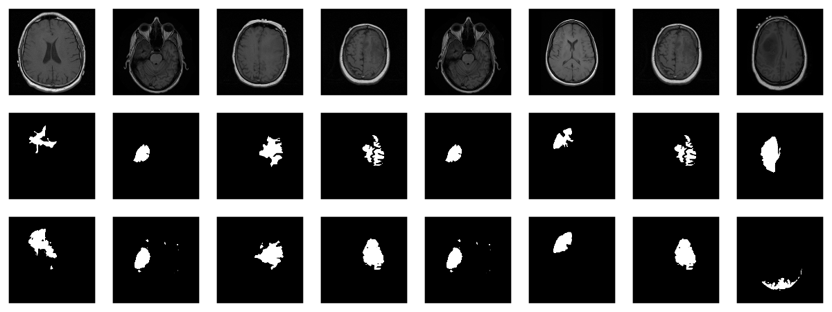
While far from perfect, most of these masks aren’t that bad
– a nice result given the small dataset!

Wrapup

This has been our most complex torch post so far; however, we
hope you’ve found the time well spent. For one, among
applications of deep learning, medical image segmentation stands
out as highly societally useful. Secondly, U-Net-like architectures
are employed in many other areas. And finally, we once more saw
torch’s flexibility and intuitive behavior in action.

Thanks for reading!