
 This tutorial is the sixth installment of introductions to the RAPIDS ecosystem.
Month: March 2021
Categories
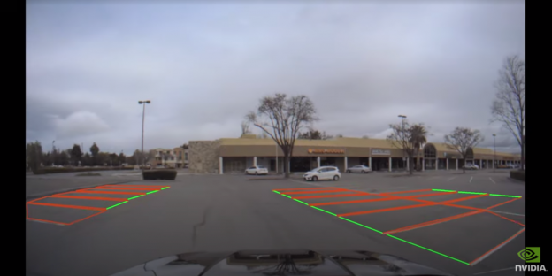
GTC 21: Top 5 Automotive Technical Sessions
 Register for the free conference to hear talks from Audi Board Member Hildegard Wortmann, Zoox CTO Jesse Levinson, University of Toronto Professor Raquel Urtasun, and Cruise SVP of Engineering Mo ElShenawy.
NVIDIA GTC is returning with a special focus on autonomous vehicles, including talks from Audi Board Member Hildegard Wortmann, Zoox CTO Jesse Levinson, University of Toronto Professor Raquel Urtasun, and Cruise SVP of Engineering Mo ElShenawy. GTC is free to attend – you and your team can register here.
This free five-day digital conference kicks off April 12 with NVIDIA CEO Jensen Huang’s keynote followed by 1,400+ talks ranging from technical deep dives to business-focused talks by C-level leaders. You won’t want to miss it.
Here are some session highlights for autonomous vehicle development:

- Deep-Sensor Fusion of Thermal and Visible Cameras for Autonomous Driving
See the latest research on fusing visual and thermal sensors for state-of-the-art segmentation accuracy in autonomous driving.
Vijay John, Assistant Professor, Toyota Technological Institute

- Understanding Safety and Security Standards for Autonomous Vehicles: An NVIDIA DRIVE Approach
Learn how to more easily integrate the NVIDIA DRIVE platform into your safe and secure AV designs with NVIDIA’s safety approach.
Karl Greb, Safety Engineering Director, NVIDIA
Riccardo Mariani, VP of Industry Safety, NVIDIA
- Autonomous Valet Parking Powered by NVIDIA DRIVE
This session will cover how Apex.AI developed a modular approach to production autonomous parking.
Dejan Pangercic, CTO, Apex.AI

- Human-Guided Autonomous Convoys
This presentation highlights the operations and challenges of deploying an autonomous convoy system for long-haul trucking.
Cetin Mericli, CEO, Locomation

- Deflating Dataset Bias Using Synthetic Data Augmentation
This session will show how targeted synthetic data augmentation can help fill gaps in static datasets for vision tasks.
Nikita Jaipuria, Research Scientist, Ford Motor Company
Additionally, from April 20-22, be sure to check out NVIDIA DRIVE Developer Days, which will consist of deep dive sessions on safe and robust AV development. These are also FREE and will be available via the GTC session catalog.
 NVIDIA CUDA-X AI are deep learning libraries for researchers and software developers to build high performance GPU-accelerated applications for conversational AI, recommendation systems and computer vision.
NVIDIA CUDA-X AI are deep learning libraries for researchers and software developers to build high performance GPU-accelerated applications for conversational AI, recommendation systems and computer vision.
Learn what’s new in the latest releases of CUDA-X AI libraries.
Refer to each package’s release notes in documentation for additional information.
NVIDIA Jarvis Open Beta
NVIDIA Jarvis is an application framework for multimodal conversational AI services that delivers real-time performance on GPUs. This version of Jarvis includes:
- ASR, NLU, and TTS models trained on thousands of hours of speech data.
- Transfer Learning Toolkit with zero coding approach to re-train on custom data.
- Fully accelerated deep learning pipelines optimized to run as scalable services.
- End-to-end workflow and tools to deploy services using one line of code.
Transfer Learning Toolkit 3.0 Developer Preview
NVIDIA released new pre-trained models for computer vision and conversational AI that can be easily fine-tuned with Transfer Learning Toolkit (TLT) 3.0 with a zero-coding approach.
Key highlights:
- New vision AI pre-trained models: license plate detection and recognition, heart rate monitoring, gesture recognition, gaze estimation, emotion recognition, face detection, and facial landmark estimation
- Newly added support for automatic speech recognition (ASR) and natural language processing (NLP)
- Choice of training with popular network architectures such as EfficientNet, YoloV4, and UNET
- Support for NVIDIA Ampere GPUs with third-generation tensor cores for performance boost
Triton Inference Server 2.7
Triton Inference Server is an open source multi-framework, cross platform inference serving software designed to simplify model production deployment. Version 2.7 includes:
- Model Analyzer – automatically finds best model configuration to maximize performance based on user-specified requirements
- Model Repo Agent API – enables custom operations to be performed to models being loaded (such as decrypting, checksumming, applying TF-TRT optimization, etc)
- Added support for ONNX Runtime backend in Triton Windows build
- Added an example Java and Scala client based on GRPC-generated API
Read full release notes here.
TensorRT 7.2 is Now Available
NVIDIA TensorRT is a platform for high-performance deep learning inference. This version of TensorRT includes:
- New Polygraphy toolkit, assists in prototyping and debugging deep learning models in various frameworks
- Support for Python 3.8
Merlin Open Beta
Merlin is an application framework and ecosystem that enables end-to-end development of recommender systems, accelerated on NVIDIA GPUs. Merlin Open Beta highlights include:
- NVTabular and HugeCTR inference support in Triton Inference Server
- Cloud configurations and cloud support (AWS/GCP)
- Dataset analysis and generation tools
- New PythonAPI for HugeCTR similar to Keras with no JSON configuration anymore
DeepStream SDK 5.1
NVIDIA DeepStream SDK is a streaming analytics toolkit for AI-based multi-sensor processing.
Key highlights for DeepStream SDK 5.1 (General Availability)
- New Python apps for using optical flow, segmentation networks, and analytics using ROI and line crossing
- Support for audio analytics with a sample application highlighting audio classifier usage
- Support for NVIDIA Ampere GPUs with third-generation tensor cores and various performance optimizations
nvJPEG2000 0.2
nvJPEG2000 is a new library for GPU-accelerated JPEG2000 image decoding. This version of nvJPEG2000 includes:
- Support for multi-tile and multi-layer decoding.
- Partial decode by specifying an area of interest for increased efficiency
- New API for commonly used GDAL interface for geospatial images
- 4x faster lossless decoding for 5-3 wavelet decoding and 7x faster loss decoding for 9-7 wavelet transform. Achieve further speed up by pipelining decoding of multiple images.
NVIDIA NeMo 1.0.0b4
NVIDIA NeMo is a toolkit to build, train and fine-tune state-of-the-art speech and language models easily. Highlights of this version include:
- Compatible with Jarvis 1.0.0b2 public beta and TLT 3.0 releases
Deep Learning Examples provide state-of-the-art reference examples that are easy to train and deploy, achieving the best reproducible accuracy and performance with NVIDIA CUDA-X AI software stack running on NVIDIA Volta, Turing, and Ampere GPUs.
New Model Scripts available from the NGC Catalog:
- nnUNet/PyT: A Self-adapting Framework for U-Net for state-of-the-art Segmentation across distinct entities, image modalities, image geometries, and dataset sizes, with no manual adjustments between datasets.
- Wide and Deep/TF2: Wide & Deep refers to a class of networks that use the output of two parts working in parallel – wide model and deep model – to make a binary prediction of CTR.
- EfficientNet PyT & TF2: A model that scales the depth, width, and resolution to achieve better performance across different datasets. EfficientNet B4 achieves state-of-the-art 82.78% top-1 accuracy on ImageNet, while being 8.4x smaller and 6.1x faster on inference than the best existing ConvNet.
- Electra: A novel pre-training method for language representations which outperforms existing techniques, given the same compute budget on a wide array of Natural Language Processing (NLP) tasks.
Natural language processing (NLP) models based on Transformers, such as BERT, RoBERTa, T5, or GPT3, are successful for a wide variety of tasks and a mainstay of modern NLP research. The versatility and robustness of Transformers are the primary drivers behind their wide-scale adoption, leading them to be easily adapted for a diverse range of sequence-based tasks — as a seq2seq model for translation, summarization, generation, and others, or as a standalone encoder for sentiment analysis, POS tagging, machine reading comprehension, etc. The key innovation in Transformers is the introduction of a self-attention mechanism, which computes similarity scores for all pairs of positions in an input sequence, and can be evaluated in parallel for each token of the input sequence, avoiding the sequential dependency of recurrent neural networks, and enabling Transformers to vastly outperform previous sequence models like LSTM.
A limitation of existing Transformer models and their derivatives, however, is that the full self-attention mechanism has computational and memory requirements that are quadratic with the input sequence length. With commonly available current hardware and model sizes, this typically limits the input sequence to roughly 512 tokens, and prevents Transformers from being directly applicable to tasks that require larger context, like question answering, document summarization or genome fragment classification. Two natural questions arise: 1) Can we achieve the empirical benefits of quadratic full Transformers using sparse models with computational and memory requirements that scale linearly with the input sequence length? 2) Is it possible to show theoretically that these linear Transformers preserve the expressivity and flexibility of the quadratic full Transformers?
We address both of these questions in a recent pair of papers. In “ETC: Encoding Long and Structured Inputs in Transformers”, presented at EMNLP 2020, we present the Extended Transformer Construction (ETC), which is a novel method for sparse attention, in which one uses structural information to limit the number of computed pairs of similarity scores. This reduces the quadratic dependency on input length to linear and yields strong empirical results in the NLP domain. Then, in “Big Bird: Transformers for Longer Sequences”, presented at NeurIPS 2020, we introduce another sparse attention method, called BigBird that extends ETC to more generic scenarios where prerequisite domain knowledge about structure present in the source data may be unavailable. Moreover, we also show that theoretically our proposed sparse attention mechanism preserves the expressivity and flexibility of the quadratic full Transformers. Our proposed methods achieve a new state of the art on challenging long-sequence tasks, including question answering, document summarization and genome fragment classification.
Attention as a Graph
The attention module used in Transformer models computes similarity scores for all pairs of positions in an input sequence. It is useful to think of the attention mechanism as a directed graph, with tokens represented by nodes and the similarity score computed between a pair of tokens represented by an edge. In this view, the full attention model is a complete graph. The core idea behind our approach is to carefully design sparse graphs, such that one only computes a linear number of similarity scores.
 |
| Full attention can be viewed as a complete graph. |
Extended Transformer Construction (ETC)
On NLP tasks that require long and structured inputs, we propose a structured sparse attention mechanism, which we call Extended Transformer Construction (ETC). To achieve structured sparsification of self attention, we developed the global-local attention mechanism. Here the input to the Transformer is split into two parts: a global input where tokens have unrestricted attention, and a long input where tokens can only attend to either the global input or to a local neighborhood. This achieves linear scaling of attention, which allows ETC to significantly scale input length.
In order to further exploit the structure of long documents, ETC combines additional ideas: representing the positional information of the tokens in a relative way, rather than using their absolute position in the sequence; using an additional training objective beyond the usual masked language model (MLM) used in models like BERT; and flexible masking of tokens to control which tokens can attend to which other tokens. For example, given a long selection of text, a global token is applied to each sentence, which connects to all tokens within the sentence, and a global token is also applied to each paragraph, which connects to all tokens within the same paragraph.
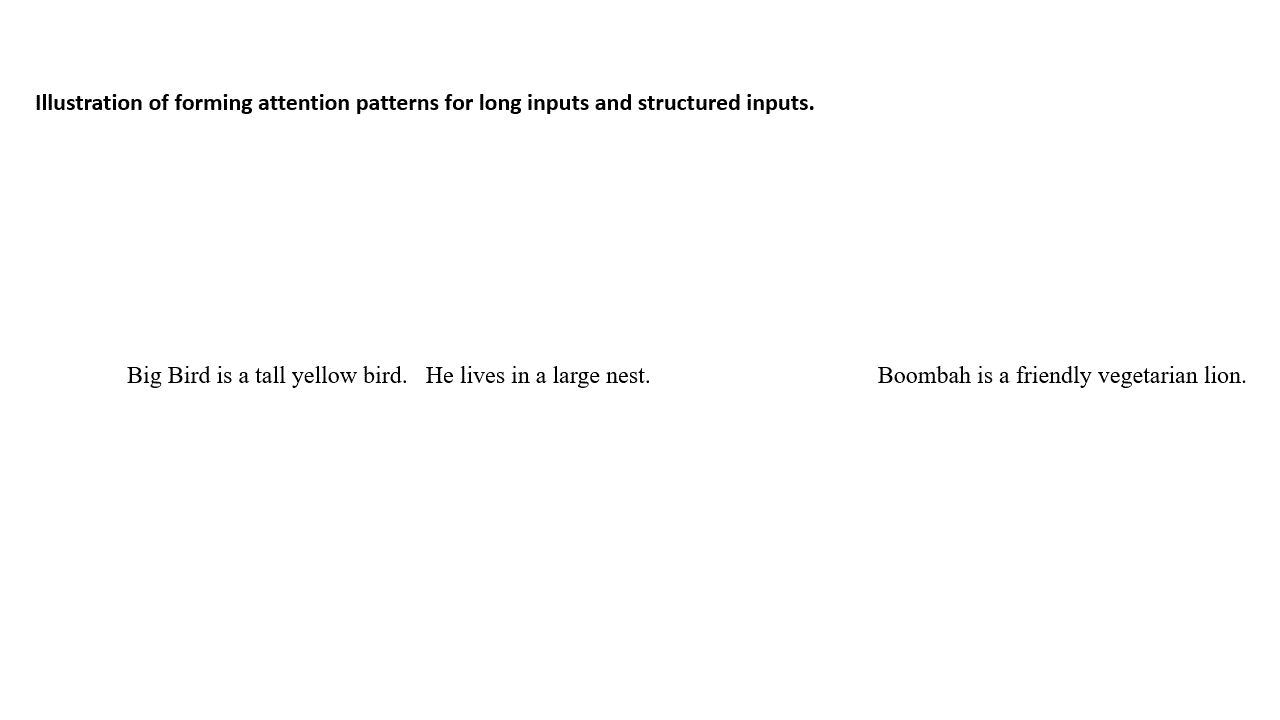 |
| An example of document structure based sparse attention of ETC model. The global variables are denoted by C (in blue) for paragraph, S (yellow) for sentence while the local variables are denoted by X (grey) for tokens corresponding to the long input. |
With this approach, we report state-of-the-art results in five challenging NLP datasets requiring long or structured inputs: TriviaQA, Natural Questions (NQ), HotpotQA, WikiHop, and OpenKP.
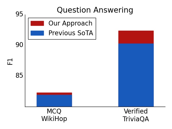 |
| Test set result on Question Answering. For both verified TriviaQA and WikiHop, using ETC achieved a new state of the art. |
BigBird
Extending the work of ETC, we propose BigBird — a sparse attention mechanism that is also linear in the number of tokens and is a generic replacement for the attention mechanism used in Transformers. In contrast to ETC, BigBird doesn’t require any prerequisite knowledge about structure present in the source data. Sparse attention in the BigBird model consists of three main parts:
- A set of global tokens attending to all parts of the input sequence
- All tokens attending to a set of local neighboring tokens
- All tokens attending to a set of random tokens
 |
| BigBird sparse attention can be seen as adding few global tokens on Watts-Strogatz graph. |
In the BigBird paper, we explain why sparse attention is sufficient to approximate quadratic attention, partially explaining why ETC was successful. A crucial observation is that there is an inherent tension between how few similarity scores one computes and the flow of information between different nodes (i.e., the ability of one token to influence each other). Global tokens serve as a conduit for information flow and we prove that sparse attention mechanisms with global tokens can be as powerful as the full attention model. In particular, we show that BigBird is as expressive as the original Transformer, is computationally universal (following the work of Yun et al. and Perez et al.), and is a universal approximator of continuous functions. Furthermore, our proof suggests that the use of random graphs can further help ease the flow of information — motivating the use of the random attention component.
This design scales to much longer sequence lengths for both structured and unstructured tasks. Further scaling can be achieved by using gradient checkpointing by trading off training time for sequence length. This lets us extend our efficient sparse transformers to include generative tasks that require an encoder and a decoder, such as long document summarization, on which we achieve a new state of the art.
 |
| Summarization ROUGE score for long documents. Both for BigPatent and ArXiv datasets, we achieve a new state of the art result. |
Moreover, the fact that BigBird is a generic replacement also allows it to be extended to new domains without pre-existing domain knowledge. In particular, we introduce a novel application of Transformer-based models where long contexts are beneficial — extracting contextual representations of genomic sequences (DNA). With longer masked language model pre-training, BigBird achieves state-of-the-art performance on downstream tasks, such as promoter-region prediction and chromatin profile prediction.
 |
| On multiple genomics tasks, such as promoter region prediction (PRP), chromatin-profile prediction including transcription factors (TF), histone-mark (HM) and DNase I hypersensitive (DHS) detection, we outperform baselines. Moreover our results show that Transformer models can be applied to multiple genomics tasks that are currently underexplored. |
Main Implementation Idea
One of the main impediments to the large scale adoption of sparse attention is the fact that sparse operations are quite inefficient in modern hardware. Behind both ETC and BigBird, one of our key innovations is to make an efficient implementation of the sparse attention mechanism. As modern hardware accelerators like GPUs and TPUs excel using coalesced memory operations, which load blocks of contiguous bytes at once, it is not efficient to have small sporadic look-ups caused by a sliding window (for local attention) or random element queries (random attention). Instead we transform the sparse local and random attention into dense tensor operations to take full advantage of modern single instruction, multiple data (SIMD) hardware.
To do this, we first “blockify” the attention mechanism to better leverage GPUs/TPUs, which are designed to operate on blocks. Then we convert the sparse attention mechanism computation into a dense tensor product through a series of simple matrix operations such as reshape, roll, and gather, as illustrated in the animation below.
 |
| Illustration of how sparse window attention is efficiently computed using roll and reshape, and without small sporadic look-ups. |
Recently, “Long Range Arena: A Benchmark for Efficient Transformers“ provided a benchmark of six tasks that require longer context, and performed experiments to benchmark all existing long range transformers. The results show that the BigBird model, unlike its counterparts, clearly reduces memory consumption without sacrificing performance.
Conclusion
We show that carefully designed sparse attention can be as expressive and flexible as the original full attention model. Along with theoretical guarantees, we provide a very efficient implementation which allows us to scale to much longer inputs. As a consequence, we achieve state-of-the-art results for question answering, document summarization and genome fragment classification. Given the generic nature of our sparse attention, the approach should be applicable to many other tasks like program synthesis and long form open domain question answering. We have open sourced the code for both ETC (github) and BigBird (github), both of which run efficiently for long sequences on both GPUs and TPUs.
Acknowledgements
This research resulted as a collaboration with Amr Ahmed, Joshua Ainslie, Chris Alberti, Vaclav Cvicek, Avinava Dubey, Zachary Fisher, Guru Guruganesh, Santiago Ontañón, Philip Pham, Anirudh Ravula, Sumit Sanghai, Qifan Wang, Li Yang, Manzil Zaheer, who co-authored EMNLP and NeurIPS papers.

 Learn how you can take advantage of the latest NVIDIA technology to enable the creation of beautiful worlds quicker and easier than ever before.
This year at GTC we have several sessions for professional content creators looking to take advantage of the latest NVIDIA technology to enable the creation of beautiful worlds quicker and easier than ever before. Find out how to add life-like realism to your projects with new ray tracing features and faster real-time volumetric rendering and simulation. Also, learn how to collaborate with creators around the world seamlessly and effortlessly no matter what software you use. We have hundreds of sessions on graphics, simulation, and design to choose from. Registration is free.
These are the five graphics sessions you can’t miss:

What’s New in OptiX
Catch up with the latest additions to the OptiX SDK and learn tips and tricks on how best to implement them into your products.

NanoVDB: A GPU-Friendly and Portable VDB Data Structure for Real-Time Rendering and Simulation
Learn how NanoVDB accelerates real-time rendering and simulation of the most graphically intensive volumetric effects on NVIDIA GPUs.

An Overview of NVIDIA CloudXR
Learn all about NVIDIA CloudXR, a groundbreaking innovation for streaming VR and AR from any OpenVR application on a remote server to a client device. Get details on the architecture of the CloudXR software stack and explore the use cases.

Building Omniverse Kit Apps and Extensions
Learn how to leverage Omniverse Kit to build amazing applications and extensions.

Making a Connector for Omniverse
Learn how to connect with the Omniverse platform, send data to it, and establish a live sync session. There will also be a USD 101 overview to get you started.
Register for free and check out GTC sessions that dive into the latest technologies for graphics and simulation. A quick registration is required to view the GTC catalog with over 1,400 free sessions covering XR, graphics, simulation, design, and more.
submitted by /u/AvisekEECS
[visit reddit] [comments]
Hi, I would like to make simple AI, which can detect hotword/wakeword and I need a lot of short audiofiles with names of chess figures. How to get the dataset like that or is there another opensource hotword/wakeword detection? (STT would be too weak and common wakeword mechanisms are deprecated or commercial ;( )
submitted by /u/Feeling_Wait_7132
[visit reddit] [comments]

Sparklyr 1.6 is now available on CRAN!
To install sparklyr 1.6 from CRAN, run
install.packages("sparklyr")
In this blog post, we shall highlight the following features and enhancements from sparklyr 1.6:
- Weighted quantile summaries
- Power iteration clustering
- spark_write_rds() + collect_from_rds()
- Dplyr-related improvements
Weighted quantile summaries
Apache Spark is well-known for supporting approximate algorithms that trade off marginal amounts of accuracy for greater speed and parallelism. Such algorithms are particularly beneficial for performing preliminary data explorations at scale, as they enable users to quickly query certain estimated statistics within a predefined error margin, while avoiding the high cost of exact computations. One example is the Greenwald-Khanna algorithm for on-line computation of quantile summaries, as described in Greenwald and Khanna (2001). This algorithm was originally designed for efficient (epsilon)- approximation of quantiles within a large dataset without the notion of data points carrying different weights, and the unweighted version of it has been implemented as approxQuantile() since Spark 2.0. However, the same algorithm can be generalized to handle weighted inputs, and as sparklyr user @Zhuk66 mentioned in this issue, a weighted version of this algorithm makes for a useful sparklyr feature.
To properly explain what weighted-quantile means, we must clarify what the weight of each data point signifies. For example, if we have a sequence of observations ((1, 1, 1, 1, 0, 2, -1, -1)), and would like to approximate the median of all data points, then we have the following two options:
-
Either run the unweighted version of approxQuantile() in Spark to scan through all 8 data points
-
Or alternatively, “compress” the data into 4 tuples of (value, weight): ((1, 0.5), (0, 0.125), (2, 0.125), (-1, 0.25)), where the second component of each tuple represents how often a value occurs relative to the rest of the observed values, and then find the median by scanning through the 4 tuples using the weighted version of the Greenwald-Khanna algorithm
We can also run through a contrived example involving the standard normal distribution to illustrate the power of weighted quantile estimation in sparklyr 1.6. Suppose we cannot simply run qnorm() in R to evaluate the quantile function of the standard normal distribution at (p = 0.25) and (p = 0.75), how can we get some vague idea about the 1st and 3rd quantiles of this distribution? One way is to sample a large number of data points from this distribution, and then apply the Greenwald-Khanna algorithm to our unweighted samples, as shown below:
library(sparklyr)

sc <- spark_connect(master = "local")

num_samples <- 1e6
samples <- data.frame(x = rnorm(num_samples))

samples_sdf <- copy_to(sc, samples, name = random_string())

samples_sdf %>%
  sdf_quantile(
    column = "x",
    probabilities = c(0.25, 0.75),
    relative.error = 0.01
  ) %>%
  print()
##        25%        75%
## -0.6629242  0.6874939
Notice that because we are working with an approximate algorithm, and have specified relative.error = 0.01, the estimated value of (-0.6629242) from above could be anywhere between the 24th and the 26th percentile of all samples. In fact, it falls in the (25.36896)-th percentile:
pnorm(-0.6629242)
## [1] 0.2536896
Now how can we make use of weighted quantile estimation from sparklyr 1.6 to obtain similar results? Simple! We can sample a large number of (x) values uniformly randomly from ((-infty, infty)) (or alternatively, just select a large number of values evenly spaced between ((-M, M)) where (M) is approximately (infty)), and assign each (x) value a weight of (displaystyle frac{1}{sqrt{2 pi}}e^{-frac{x^2}{2}}), the standard normal distribution’s probability density at (x). Finally, we run the weighted version of sdf_quantile() from sparklyr 1.6, as shown below:
library(sparklyr)

sc <- spark_connect(master = "local")

num_samples <- 1e6
M <- 1000
samples <- tibble::tibble(
  x = M * seq(-num_samples / 2 + 1, num_samples / 2) / num_samples,
  weight = dnorm(x)
)

samples_sdf <- copy_to(sc, samples, name = random_string())

samples_sdf %>%
  sdf_quantile(
    column = "x",
    weight.column = "weight",
    probabilities = c(0.25, 0.75),
    relative.error = 0.01
  ) %>%
  print()
##    25%    75%
## -0.696  0.662
Voilà! The estimates are not too far off from the 25th and 75th percentiles (in relation to our abovementioned maximum permissible error of (0.01)):
pnorm(-0.696)
## [1] 0.2432144
pnorm(0.662)
## [1] 0.7460144
Power iteration clustering
Power iteration clustering (PIC), a simple and scalable graph clustering method presented in Lin and Cohen (2010), first finds a low-dimensional embedding of a dataset, using truncated power iteration on a normalized pairwise-similarity matrix of all data points, and then uses this embedding as the “cluster indicator”, an intermediate representation of the dataset that leads to fast convergence when used as input to k-means clustering. This process is very well illustrated in figure 1 of Lin and Cohen (2010) (reproduced below)
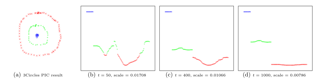
in which the leftmost image is the visualization of a dataset consisting of 3 circles, with points colored in red, green, and blue indicating clustering results, and the subsequent images show the power iteration process gradually transforming the original set of points into what appears to be three disjoint line segments, an intermediate representation that can be rapidly separated into 3 clusters using k-means clustering with (k = 3).
In sparklyr 1.6, ml_power_iteration() was implemented to make the PIC functionality in Spark accessible from R. It expects as input a 3-column Spark dataframe that represents a pairwise-similarity matrix of all data points. Two of the columns in this dataframe should contain 0-based row and column indices, and the third column should hold the corresponding similarity measure. In the example below, we will see a dataset consisting of two circles being easily separated into two clusters by ml_power_iteration(), with the Gaussian kernel being used as the similarity measure between any 2 points:
gen_similarity_matrix <- function() {
  # Guassian similarity measure
  guassian_similarity <- function(pt1, pt2) {
    exp(-sum((pt2 - pt1) ^ 2) / 2)
  }
  # generate evenly distributed points on a circle centered at the origin
  gen_circle <- function(radius, num_pts) {
    seq(0, num_pts - 1) %>%
      purrr::map_dfr(
        function(idx) {
          theta <- 2 * pi * idx / num_pts
          radius * c(x = cos(theta), y = sin(theta))
        })
  }
  # generate points on both circles
  pts <- rbind(
    gen_circle(radius = 1, num_pts = 80),
    gen_circle(radius = 4, num_pts = 80)
  )
  # populate the pairwise similarity matrix (stored as a 3-column dataframe)
  similarity_matrix <- data.frame()
  for (i in seq(2, nrow(pts)))
    similarity_matrix <- similarity_matrix %>%
      rbind(seq(i - 1L) %>%
        purrr::map_dfr(~ list(
          src = i - 1L, dst = .x - 1L,
          similarity = guassian_similarity(pts[i,], pts[.x,])
        ))
      )

  similarity_matrix
}

library(sparklyr)

sc <- spark_connect(master = "local")
sdf <- copy_to(sc, gen_similarity_matrix())
clusters <- ml_power_iteration(
  sdf, k = 2, max_iter = 10, init_mode = "degree",
  src_col = "src", dst_col = "dst", weight_col = "similarity"
)

clusters %>% print(n = 160)
## # A tibble: 160 x 2
##        id cluster
##     <dbl>   <int>
##   1     0       1
##   2     1       1
##   3     2       1
##   4     3       1
##   5     4       1
##   ...
##   157   156       0
##   158   157       0
##   159   158       0
##   160   159       0
The output shows points from the two circles being assigned to separate clusters, as expected, after only a small number of PIC iterations.
spark_write_rds() + collect_from_rds()
spark_write_rds() and collect_from_rds() are implemented as a less memory- consuming alternative to collect(). Unlike collect(), which retrieves all elements of a Spark dataframe through the Spark driver node, hence potentially causing slowness or out-of-memory failures when collecting large amounts of data, spark_write_rds(), when used in conjunction with collect_from_rds(), can retrieve all partitions of a Spark dataframe directly from Spark workers, rather than through the Spark driver node. First, spark_write_rds() will distribute the tasks of serializing Spark dataframe partitions in RDS version 2 format among Spark workers. Spark workers can then process multiple partitions in parallel, each handling one partition at a time and persisting the RDS output directly to disk, rather than sending dataframe partitions to the Spark driver node. Finally, the RDS outputs can be re-assembled to R dataframes using collect_from_rds().
Shown below is an example of spark_write_rds() + collect_from_rds() usage, where RDS outputs are first saved to HDFS, then downloaded to the local filesystem with hadoop fs -get, and finally, post-processed with collect_from_rds():
library(sparklyr)
library(nycflights13)

num_partitions <- 10L
sc <- spark_connect(master = "yarn", spark_home = "/usr/lib/spark")
flights_sdf <- copy_to(sc, flights, repartition = num_partitions)

# Spark workers serialize all partition in RDS format in parallel and write RDS
# outputs to HDFS
spark_write_rds(
  flights_sdf,
  dest_uri = "hdfs://<namenode>:8020/flights-part-{partitionId}.rds"
)

# Run `hadoop fs -get` to download RDS files from HDFS to local file system
for (partition in seq(num_partitions) - 1)
  system2(
    "hadoop",
    c("fs", "-get", sprintf("hdfs://<namenode>:8020/flights-part-%d.rds", partition))
  )

# Post-process RDS outputs
partitions <- seq(num_partitions) - 1 %>%
  lapply(function(partition) collect_from_rds(sprintf("flights-part-%d.rds", partition)))

# Optionally, call `rbind()` to combine data from all partitions into a single R dataframe
flights_df <- do.call(rbind, partitions)
Dplyr-related improvements
Similar to other recent sparklyr releases, sparklyr 1.6 comes with a number of dplyr-related improvements, such as
- Support for where() predicate within select() and summarize(across(…)) operations on Spark dataframes
- Addition of if_all() and if_any() functions
- Full compatibility with dbplyr 2.0 backend API
select(where(…)) and summarize(across(where(…)))
The dplyr where(…) construct is useful for applying a selection or aggregation function to multiple columns that satisfy some boolean predicate. For example,
library(dplyr)

iris %>% select(where(is.numeric))
returns all numeric columns from the iris dataset, and
library(dplyr)

iris %>% summarize(across(where(is.numeric), mean))
computes the average of each numeric column.
In sparklyr 1.6, both types of operations can be applied to Spark dataframes, e.g.,
library(dplyr)
library(sparklyr)

sc <- spark_connect(master = "local")
iris_sdf <- copy_to(sc, iris, name = random_string())

iris_sdf %>% select(where(is.numeric))

iris %>% summarize(across(where(is.numeric), mean))
if_all() and if_any()
if_all() and if_any() are two convenience functions from dplyr 1.0.4 (see here for more details) that effectively1 combine the results of applying a boolean predicate to a tidy selection of columns using the logical and/or operators.
Starting from sparklyr 1.6, if_all() and if_any() can also be applied to Spark dataframes, .e.g.,
library(dplyr)
library(sparklyr)

sc <- spark_connect(master = "local")
iris_sdf <- copy_to(sc, iris, name = random_string())

# Select all records with Petal.Width > 2 and Petal.Length > 2
iris_sdf %>% filter(if_all(starts_with("Petal"), ~ .x > 2))

# Select all records with Petal.Width > 5 or Petal.Length > 5
iris_sdf %>% filter(if_any(starts_with("Petal"), ~ .x > 5))
Compatibility with dbplyr 2.0 backend API
Sparklyr 1.6 is fully compatible with the newer dbplyr 2.0 backend API (by implementing all interface changes recommended in here), while still maintaining backward compatibility with the previous edition of dbplyr API, so that sparklyr users will not be forced to switch to any particular version of dbplyr.
This should be a mostly non-user-visible change as of now. In fact, the only discernible behavior change will be the following code
library(dbplyr)
library(sparklyr)

sc <- spark_connect(master = "local")

print(dbplyr_edition(sc))
outputting
[1] 2
if sparklyr is working with dbplyr 2.0+, and
[1] 1
if otherwise.
Acknowledgements
In chronological order, we would like to thank the following contributors for making sparklyr 1.6 awesome:
- @yitao-li
- @pgramme
- @javierluraschi
- @andrew-christianson
- @jozefhajnala
- @nathaneastwood
- [@mzorko] (https://github.com/mzorko)
We would also like to give a big shout-out to the wonderful open-source community behind sparklyr, without whom we would not have benefitted from numerous sparklyr-related bug reports and feature suggestions.
Finally, the author of this blog post also very much appreciates the highly valuable editorial suggestions from @skeydan.
If you wish to learn more about sparklyr, we recommend checking out sparklyr.ai, spark.rstudio.com, and also some previous sparklyr release posts such as sparklyr 1.5 and sparklyr 1.4.
That is all. Thanks for reading!
Greenwald, Michael, and Sanjeev Khanna. 2001. “Space-Efficient Online Computation of Quantile Summaries.” SIGMOD Rec. 30 (2): 58–66. https://doi.org/10.1145/376284.375670.
Lin, Frank, and William Cohen. 2010. “Power Iteration Clustering.” In, 655–62.
-
modulo possible implementation-dependent short-circuit evaluations↩︎
Sparklyr 1.6 is now available on CRAN!
To install sparklyr 1.6 from CRAN, run
install.packages("sparklyr")
In this blog post, we shall highlight the following features and enhancements from sparklyr 1.6:
- Weighted quantile summaries
- Power iteration clustering
- spark_write_rds() + collect_from_rds()
- Dplyr-related improvements
Weighted quantile summaries
Apache Spark is well-known for supporting approximate algorithms that trade off marginal amounts of accuracy for greater speed and parallelism. Such algorithms are particularly beneficial for performing preliminary data explorations at scale, as they enable users to quickly query certain estimated statistics within a predefined error margin, while avoiding the high cost of exact computations. One example is the Greenwald-Khanna algorithm for on-line computation of quantile summaries, as described in Greenwald and Khanna (2001). This algorithm was originally designed for efficient (epsilon)- approximation of quantiles within a large dataset without the notion of data points carrying different weights, and the unweighted version of it has been implemented as approxQuantile() since Spark 2.0. However, the same algorithm can be generalized to handle weighted inputs, and as sparklyr user @Zhuk66 mentioned in this issue, a weighted version of this algorithm makes for a useful sparklyr feature.
To properly explain what weighted-quantile means, we must clarify what the weight of each data point signifies. For example, if we have a sequence of observations ((1, 1, 1, 1, 0, 2, -1, -1)), and would like to approximate the median of all data points, then we have the following two options:
-
Either run the unweighted version of approxQuantile() in Spark to scan through all 8 data points
-
Or alternatively, “compress” the data into 4 tuples of (value, weight): ((1, 0.5), (0, 0.125), (2, 0.125), (-1, 0.25)), where the second component of each tuple represents how often a value occurs relative to the rest of the observed values, and then find the median by scanning through the 4 tuples using the weighted version of the Greenwald-Khanna algorithm
We can also run through a contrived example involving the standard normal distribution to illustrate the power of weighted quantile estimation in sparklyr 1.6. Suppose we cannot simply run qnorm() in R to evaluate the quantile function of the standard normal distribution at (p = 0.25) and (p = 0.75), how can we get some vague idea about the 1st and 3rd quantiles of this distribution? One way is to sample a large number of data points from this distribution, and then apply the Greenwald-Khanna algorithm to our unweighted samples, as shown below:
library(sparklyr)

sc <- spark_connect(master = "local")

num_samples <- 1e6
samples <- data.frame(x = rnorm(num_samples))

samples_sdf <- copy_to(sc, samples, name = random_string())

samples_sdf %>%
  sdf_quantile(
    column = "x",
    probabilities = c(0.25, 0.75),
    relative.error = 0.01
  ) %>%
  print()
##        25%        75%
## -0.6629242  0.6874939
Notice that because we are working with an approximate algorithm, and have specified relative.error = 0.01, the estimated value of (-0.6629242) from above could be anywhere between the 24th and the 26th percentile of all samples. In fact, it falls in the (25.36896)-th percentile:
pnorm(-0.6629242)
## [1] 0.2536896
Now how can we make use of weighted quantile estimation from sparklyr 1.6 to obtain similar results? Simple! We can sample a large number of (x) values uniformly randomly from ((-infty, infty)) (or alternatively, just select a large number of values evenly spaced between ((-M, M)) where (M) is approximately (infty)), and assign each (x) value a weight of (displaystyle frac{1}{sqrt{2 pi}}e^{-frac{x^2}{2}}), the standard normal distribution’s probability density at (x). Finally, we run the weighted version of sdf_quantile() from sparklyr 1.6, as shown below:
library(sparklyr)

sc <- spark_connect(master = "local")

num_samples <- 1e6
M <- 1000
samples <- tibble::tibble(
  x = M * seq(-num_samples / 2 + 1, num_samples / 2) / num_samples,
  weight = dnorm(x)
)

samples_sdf <- copy_to(sc, samples, name = random_string())

samples_sdf %>%
  sdf_quantile(
    column = "x",
    weight.column = "weight",
    probabilities = c(0.25, 0.75),
    relative.error = 0.01
  ) %>%
  print()
##    25%    75%
## -0.696  0.662
Voilà! The estimates are not too far off from the 25th and 75th percentiles (in relation to our abovementioned maximum permissible error of (0.01)):
pnorm(-0.696)
## [1] 0.2432144
pnorm(0.662)
## [1] 0.7460144
Power iteration clustering
Power iteration clustering (PIC), a simple and scalable graph clustering method presented in Lin and Cohen (2010), first finds a low-dimensional embedding of a dataset, using truncated power iteration on a normalized pairwise-similarity matrix of all data points, and then uses this embedding as the “cluster indicator”, an intermediate representation of the dataset that leads to fast convergence when used as input to k-means clustering. This process is very well illustrated in figure 1 of Lin and Cohen (2010) (reproduced below)
in which the leftmost image is the visualization of a dataset consisting of 3 circles, with points colored in red, green, and blue indicating clustering results, and the subsequent images show the power iteration process gradually transforming the original set of points into what appears to be three disjoint line segments, an intermediate representation that can be rapidly separated into 3 clusters using k-means clustering with (k = 3).
In sparklyr 1.6, ml_power_iteration() was implemented to make the PIC functionality in Spark accessible from R. It expects as input a 3-column Spark dataframe that represents a pairwise-similarity matrix of all data points. Two of the columns in this dataframe should contain 0-based row and column indices, and the third column should hold the corresponding similarity measure. In the example below, we will see a dataset consisting of two circles being easily separated into two clusters by ml_power_iteration(), with the Gaussian kernel being used as the similarity measure between any 2 points:
gen_similarity_matrix <- function() {
  # Guassian similarity measure
  guassian_similarity <- function(pt1, pt2) {
    exp(-sum((pt2 - pt1) ^ 2) / 2)
  }
  # generate evenly distributed points on a circle centered at the origin
  gen_circle <- function(radius, num_pts) {
    seq(0, num_pts - 1) %>%
      purrr::map_dfr(
        function(idx) {
          theta <- 2 * pi * idx / num_pts
          radius * c(x = cos(theta), y = sin(theta))
        })
  }
  # generate points on both circles
  pts <- rbind(
    gen_circle(radius = 1, num_pts = 80),
    gen_circle(radius = 4, num_pts = 80)
  )
  # populate the pairwise similarity matrix (stored as a 3-column dataframe)
  similarity_matrix <- data.frame()
  for (i in seq(2, nrow(pts)))
    similarity_matrix <- similarity_matrix %>%
      rbind(seq(i - 1L) %>%
        purrr::map_dfr(~ list(
          src = i - 1L, dst = .x - 1L,
          similarity = guassian_similarity(pts[i,], pts[.x,])
        ))
      )

  similarity_matrix
}

library(sparklyr)

sc <- spark_connect(master = "local")
sdf <- copy_to(sc, gen_similarity_matrix())
clusters <- ml_power_iteration(
  sdf, k = 2, max_iter = 10, init_mode = "degree",
  src_col = "src", dst_col = "dst", weight_col = "similarity"
)

clusters %>% print(n = 160)
## # A tibble: 160 x 2
##        id cluster
##     <dbl>   <int>
##   1     0       1
##   2     1       1
##   3     2       1
##   4     3       1
##   5     4       1
##   ...
##   157   156       0
##   158   157       0
##   159   158       0
##   160   159       0
The output shows points from the two circles being assigned to separate clusters, as expected, after only a small number of PIC iterations.
spark_write_rds() + collect_from_rds()
spark_write_rds() and collect_from_rds() are implemented as a less memory- consuming alternative to collect(). Unlike collect(), which retrieves all elements of a Spark dataframe through the Spark driver node, hence potentially causing slowness or out-of-memory failures when collecting large amounts of data, spark_write_rds(), when used in conjunction with collect_from_rds(), can retrieve all partitions of a Spark dataframe directly from Spark workers, rather than through the Spark driver node. First, spark_write_rds() will distribute the tasks of serializing Spark dataframe partitions in RDS version 2 format among Spark workers. Spark workers can then process multiple partitions in parallel, each handling one partition at a time and persisting the RDS output directly to disk, rather than sending dataframe partitions to the Spark driver node. Finally, the RDS outputs can be re-assembled to R dataframes using collect_from_rds().
Shown below is an example of spark_write_rds() + collect_from_rds() usage, where RDS outputs are first saved to HDFS, then downloaded to the local filesystem with hadoop fs -get, and finally, post-processed with collect_from_rds():
library(sparklyr)
library(nycflights13)

num_partitions <- 10L
sc <- spark_connect(master = "yarn", spark_home = "/usr/lib/spark")
flights_sdf <- copy_to(sc, flights, repartition = num_partitions)

# Spark workers serialize all partition in RDS format in parallel and write RDS
# outputs to HDFS
spark_write_rds(
  flights_sdf,
  dest_uri = "hdfs://<namenode>:8020/flights-part-{partitionId}.rds"
)

# Run `hadoop fs -get` to download RDS files from HDFS to local file system
for (partition in seq(num_partitions) - 1)
  system2(
    "hadoop",
    c("fs", "-get", sprintf("hdfs://<namenode>:8020/flights-part-%d.rds", partition))
  )

# Post-process RDS outputs
partitions <- seq(num_partitions) - 1 %>%
  lapply(function(partition) collect_from_rds(sprintf("flights-part-%d.rds", partition)))

# Optionally, call `rbind()` to combine data from all partitions into a single R dataframe
flights_df <- do.call(rbind, partitions)
Dplyr-related improvements
Similar to other recent sparklyr releases, sparklyr 1.6 comes with a number of dplyr-related improvements, such as
- Support for where() predicate within select() and summarize(across(…)) operations on Spark dataframes
- Addition of if_all() and if_any() functions
- Full compatibility with dbplyr 2.0 backend API
select(where(…)) and summarize(across(where(…)))
The dplyr where(…) construct is useful for applying a selection or aggregation function to multiple columns that satisfy some boolean predicate. For example,
library(dplyr)

iris %>% select(where(is.numeric))
returns all numeric columns from the iris dataset, and
library(dplyr)

iris %>% summarize(across(where(is.numeric), mean))
computes the average of each numeric column.
In sparklyr 1.6, both types of operations can be applied to Spark dataframes, e.g.,
library(dplyr)
library(sparklyr)

sc <- spark_connect(master = "local")
iris_sdf <- copy_to(sc, iris, name = random_string())

iris_sdf %>% select(where(is.numeric))

iris %>% summarize(across(where(is.numeric), mean))
if_all() and if_any()
if_all() and if_any() are two convenience functions from dplyr 1.0.4 (see here for more details) that effectively1 combine the results of applying a boolean predicate to a tidy selection of columns using the logical and/or operators.
Starting from sparklyr 1.6, if_all() and if_any() can also be applied to Spark dataframes, .e.g.,
library(dplyr)
library(sparklyr)

sc <- spark_connect(master = "local")
iris_sdf <- copy_to(sc, iris, name = random_string())

# Select all records with Petal.Width > 2 and Petal.Length > 2
iris_sdf %>% filter(if_all(starts_with("Petal"), ~ .x > 2))

# Select all records with Petal.Width > 5 or Petal.Length > 5
iris_sdf %>% filter(if_any(starts_with("Petal"), ~ .x > 5))
Compatibility with dbplyr 2.0 backend API
Sparklyr 1.6 is fully compatible with the newer dbplyr 2.0 backend API (by implementing all interface changes recommended in here), while still maintaining backward compatibility with the previous edition of dbplyr API, so that sparklyr users will not be forced to switch to any particular version of dbplyr.
This should be a mostly non-user-visible change as of now. In fact, the only discernible behavior change will be the following code
library(dbplyr)
library(sparklyr)

sc <- spark_connect(master = "local")

print(dbplyr_edition(sc))
outputting
[1] 2
if sparklyr is working with dbplyr 2.0+, and
[1] 1
if otherwise.
Acknowledgements
In chronological order, we would like to thank the following contributors for making sparklyr 1.6 awesome:
- @yitao-li
- @pgramme
- @javierluraschi
- @andrew-christianson
- @jozefhajnala
- @nathaneastwood
- [@mzorko] (https://github.com/mzorko)
We would also like to give a big shout-out to the wonderful open-source community behind sparklyr, without whom we would not have benefitted from numerous sparklyr-related bug reports and feature suggestions.
Finally, the author of this blog post also very much appreciates the highly valuable editorial suggestions from @skeydan.
If you wish to learn more about sparklyr, we recommend checking out sparklyr.ai, spark.rstudio.com, and also some previous sparklyr release posts such as sparklyr 1.5 and sparklyr 1.4.
That is all. Thanks for reading!
Greenwald, Michael, and Sanjeev Khanna. 2001. “Space-Efficient Online Computation of Quantile Summaries.” SIGMOD Rec. 30 (2): 58–66. https://doi.org/10.1145/376284.375670.
Lin, Frank, and William Cohen. 2010. “Power Iteration Clustering.” In, 655–62.
-
modulo possible implementation-dependent short-circuit evaluations↩︎
Categories
Come Sale Away with GFN Thursday
GFN Thursday means more games for GeForce NOW members, every single week. This week’s list includes the day-and-date release of Spacebase Startopia, but first we want to share the scoop on some fantastic sales available across our digital game store partners that members will want to take advantage of this very moment. Discounts for All Read article >
The post Come Sale Away with GFN Thursday appeared first on The Official NVIDIA Blog.