Accelerating the Wide & Deep Model Workflow from 25 Hours to 10 Minutes Using NVIDIA GPUs

Recommender systems drive engagement on many of the most popular online platforms. As data volume grows exponentially, data scientists increasingly turn from traditional machine learning methods to highly expressive, deep learning models to improve recommendation quality. Often, the recommendations are framed as modeling the completion of a user-item matrix, in which the user-item entry is … Continued

Most current online recommender systems are implicit rating-based, clickthrough rate (CTR) prediction tasks. The model estimates the probability of positive action (click), given user and item characteristics. One of the most popular DNN-based methods is Google’s Wide & Deep Learning for Recommender Systems, which has emerged as a general tool for solving CTR prediction tasks, thanks to its power of generalization (Deep) and memorization (Wide).

The Wide & Deep model falls into a category of content-based recommender models that are like Facebook’s deep learning recommendation model (DLRM), where input to the model consists of characteristics of the User and Item and the output is some form of rating.

In this post, we detail the new TensorFlow2 implementation of the Wide & Deep model that was recently added to the NVIDIA Deep Learning Examples repository. It provides the end-to-end training for easily reproducible results in training the model, using the Kaggle Outbrain Click Prediction Challenge dataset. This implementation touches on two important aspects of building recommender systems: dataset preprocessing and model training.

First, we introduce the Wide & Deep model and the dataset. Then, we give details on the preprocessing completed in two variants, CPU and GPU. Finally, we discuss aspects of model convergence, training stability, and performance, both for training and evaluation.

Wide & Deep model overview

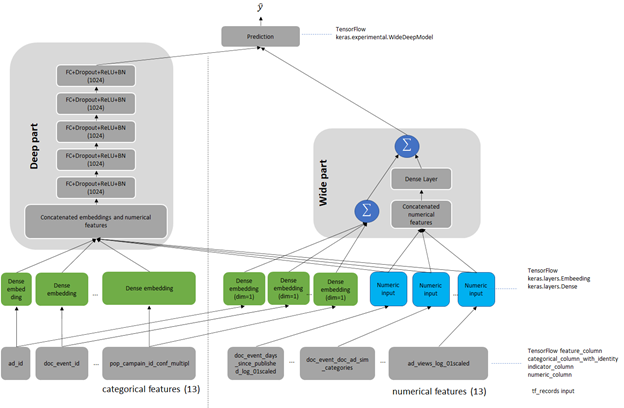
Wide & Deep refers to a class of networks that use the output of two parts working in parallel—a wide model and a deep model—to make binary prediction of CTR. The wide part is a linear model of features together with their transforms, responsible for the memorization of feature interactions. The deep part is a series of fully connected layers, allowing the model better generalization for unseen cross-features interactions. The model can handle both numerical continuous features as well as categorical features represented as dense embeddings. Figure 1 shows the architecture of the model. We changed the size of the deep part from the original of 1024, 512, 256 into five fully connected layers of 1024 neurons.

Architecture shows categorical features and numerical features of the model. — *Figure 1. The architecture of the Wide & Deep model*.

Outbrain dataset

The original Wide & Deep paper trains on the Google Play dataset. Because this data is proprietary to Google, we chose a publicly available dataset for easy reproduction. As a reference dataset, we used the Kaggle Outbrain Click Prediction Challenge data. This dataset is preprocessed to obtain a subset of the features engineered by the 19th-place finisher in the Kaggle Outbrain Click Prediction Challenge. This competition challenged competitors to predict the likelihood of a clickthrough for a particular website ad. Competitors were given information about the user, display, document, and ad to train their models. For more information, see Outbrain Click Prediction.

The Outbrain dataset is preprocessed to get feature input for the model. Each sample in the dataset consists of features of the Request (User) and Item, together with a binary output label. Request-level features describe the person and context to which to make recommendations, whereas Item-level features describe those objects to consider recommending. In the Outbrain dataset, these are ads. Request– and Item-level features contain both numerical features that you can input directly to the network. Categorical variables are represented as trainable embeddings of various dimensions. For more information about feature counts, cardinalities, embedding dimensions, and other dataset characteristics, see the WideAndDeep readme file on GitHub.

Preprocessing

As in every other recommender system, preprocessing is a key for efficient recommendation here. We present and compare two dataset preprocessing workflows: Spark-CPU and NVTabular GPU. Both produce datasets of the same number, type, and meaning of features so that the model is agnostic to the type of dataset preprocessing used. The presented preprocessing aims to produce the dataset in a form of pre-batched TFRecords to be consumed by the data loader during model training.

Scope of preprocessing

The preprocessing is described in detail in the readme of the Deep Learning Examples repository. In this post, we give only the outlook on the scope of data wrangling to create the final 26 features: 13 categorical and 13 numerical, obtained from the original Outbrain dataset. Both of the workflows consist of the following operations:

Separating out the validation set for cross-validation.
Filling missing data with mode, median, or imputed values.
Joining click data, ad metadata, and document category, topic, and entity tables to create an enriched table.
Computing seven CTRs for ads grouped by seven features.
Computing the attribute cosine similarity between the landing page and featured ad.
Math transformations of the numeric features (logarithmic, scaling, and binning).
Categorizing data using hash-bucketing.
Storing the resulting set of features in pre-batched TFRecord format.

Comparison of preprocessing workflows

To compare the NVTabular and Spark workflows, we built both from a known-good Spark-CPU workflow, included in the NVIDIA Wide & Deep TensorFlow 2 GitHub repository. For simplicity, we limited the number of dataset features to calculate during preprocessing. We chose the most common ones used in recommender systems that both workflows (Spark and NVTabular) support. Because NVTabular is a relatively new framework still in active development, we limited the scope of comparison to features supported by the NVTabular library.

When comparing Spark and NVTabular, we extracted the most important metrics that influence the choice of framework in target preprocessing. Table 1 presents a snapshot comparison of two types of preprocessing using the following metrics:

Threshold result. The necessity of achieving MAP@12 greater than the arbitrary chosen threshold of 0.655 for the Outbrain dataset.
Source code lines. The lines needed to achieve the set of features that the model uses for training. This single metric tries to capture how difficult it is to create and maintain the production code. It also gives an intuition about the level of difficulty when experimenting with adding new dataset features or changing existing ones.
Total RAM consumption. This estimates the size and type of machine needed to perform preprocessing.
Preprocessing time that is critical for recommender systems. In production environments where you must retrain the model with new data, this metric is strictly bounded with the necessity of dataset preprocessing. You can remove a too-long preprocessing time for some applications. When that time is short, you can even include the preprocessing in end-to-end training. Test the hypothesis of variable importance with the hyperparameter tuning of the network.

We did not enforce 1:1 parity between the datasets, as convergence accuracy proves the validity of the features.

	CPU preprocessing: Spark on NVIDIA DGX-1	CPU preprocessing: Spark on NVIDIA DGX A100	GPU preprocessing: NVTabular on DGX-1 8-GPU	GPU preprocessing: NVTabular DGX A100 8-GPU
Lines of code	~1,500	~1,500	~500	~500
Top RAM consumption [GB]	167.0	223.4	48.7	50.6
Top VRAM consumption per GPU [GB]	0	0	13	67
Preprocessing time [min]	45.6	38.5	3.9	2.3

Table 1. A comparison of CPU preprocessing (Spark) and GPU preprocessing (NVTabular).

Convergence accuracy

On the chosen metric for the Outbrain dataset, Mean Average Precision at 12 (MAP@12), both the features produced by Spark-CPU and NVTabular achieve similar convergence accuracy, MAP@12>0.655.

Hardware requirements

You can run the NVTabular and Spark-CPU versions on DGX-1 V100 and DGX A100 supercomputers. Spark-CPU consumes around 170 GB of RAM while the RAM footprint of NVTabular is about 3x smaller. NVTabular can run successively even on a single-GPU machine and still be an order of magnitude faster than Spark-CPU without the need of memory-optimized computers.

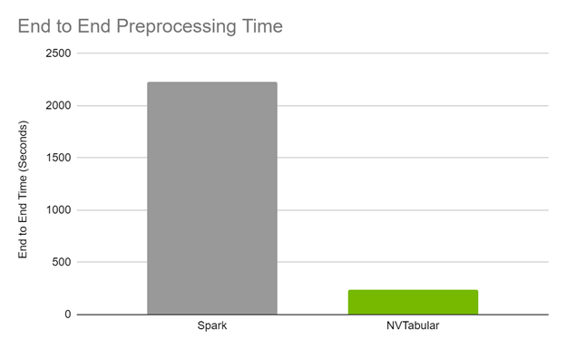
End-to-end preprocessing time

The end-to-end preprocessing time is 17x faster on GPU for DGX A100 and 12x on GPU on DGX-1 comparing Spark CPU and NVTabular GPU preprocessing.

Bar chart shows that NVTabular processing time is much faster than Spark. — *Figure 2. Outbrain dataset preprocessing time comparison.*

Code brevity and legibility

The Spark code to generate the features spans over approximately 1,500 lines, while the NVTabular code is about 500 lines. The brevity in the NVTabular workflow also lends itself to legibility, as fewer lines of code and descriptive function signatures make it obvious what a given line is trying to accomplish.

The following list contains samples with side-to-side comparisons of Spark and NVTabular, showing the increase of code brevity and legibility in favor of NVTabular. The operation used in both is taking the TF-IDF cosine similarity between an ad and its landing page.

Model training and evaluation

Training the model is analyzed based on the following criteria:

Reaching evaluation metrics.
Fast and stable training (forward and backward pass): Constantly reaching an evaluation metric not dependent on initialization, hardware architecture, or other training features.
Fast scoring of the evaluation set: Reaching performance throughput to mimic model’s behavior in production.

We used the Mean Average Precision at 12 (MAP@12) metric, the same as used in the original Outbrain Kaggle competition. Direct comparison of the obtained accuracies is unjustified because, for the original Kaggle competition, there were data leaks that could be artificially used for post-processing of model results, resulting in higher MAP@12 score.

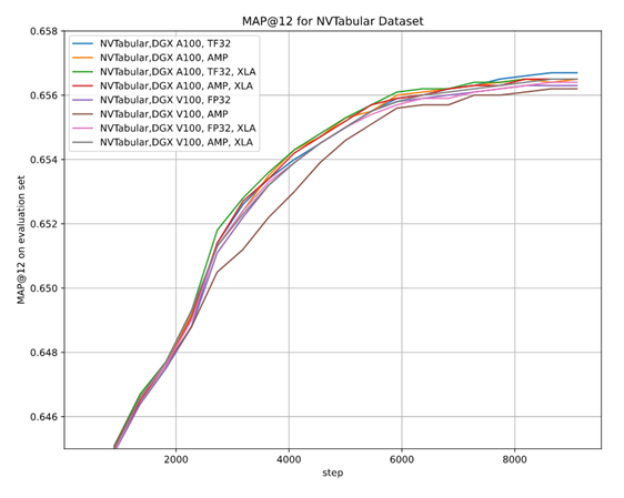
*Figure 3. Learning curve of Wide & Deep model for NVTabular dataset for multiple training setups.*

As there are multiple options for setups—two hardware architectures (A100 and V100), multiple floating-point number precisions (FP32, TF32, AMP), two versions of preprocessing (Spark-CPU and NVTabular), and the XLA optimizer, it is essential to be sure that the convergence is achieved in each setup. We performed multiple stability tests for accuracy that prove achieving MAP@12 above the selected threshold, regardless of training setup, training stability, and the impact of AMP on accuracy.

Training performance results

As stated earlier, we wanted the model to be fast in training. You can measure this in two ways: by the model throughput [samples/s] and time to train [min]. When training on CPU compared to GPU, you can experience speedups up to 108x for the NVIDIA Ampere Architecture and TF32 precision (Figure 4).

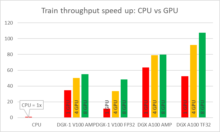
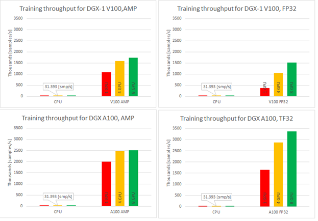
Speedup of CPU vs GPU training. CPU is 1x. — *Figure 4. Training throughput speedup of GPU vs. CPU training.*

Speedup of CPU vs GPU training is up to over 100x. — *Figure 5. Training throughput for DGX-1 V100 and DGX A100 for AMP and FP32/TF32 precision for 1, 4, and 8 GPUs. Shown numbers are for XLA on.*

Single-GPU configurations experience up to 1.2x speedup while using AMP for Ampere architecture. This number is even better for Volta, where the speedup is over 3x. Introducing multi-GPU training in a strong scaling mode ends up in speedups of 1.2x–4.6x in comparison to single-GPU training. Comparison of Ampere and Volta architectures for FP32 and TF32 training, respectively, shows a speedup of 2.2x (single GPU) to 4.5x (eight GPUs). Ampere is also 1.4x– 1.8x faster than Volta for AMP training. Bearing in mind that you don’t lose any accuracy with AMP, XLA and multi-GPU, this brings a huge value to recommender systems models.

Training time improves significantly when training on GPU in comparison to CPU and for best configuration is faster over 100x. TFRecords dataset consumes around 40GB of disk space. For best configuration of training (8x A100, TF32 precision, XLA on) this implementation of the Wide & Deep model performs a 20-epoch training within eight minutes, resulting in less than 25[s] per epoch during training.

Evaluating performance results

Having a model that trains with such throughput is beneficial. In fact, in offline scenarios, another parameter is important: how fast you can evaluate all pairs of users and items. If you have 10⁶ distinct users and only 10³ distinct items, that gives you 10⁹ different user-item pairs. Fast evaluation on training models is a key concept. Figure 6 shows the evaluation performance for A100 and V100 varying batch size.

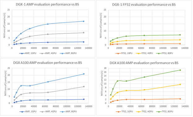
Evaluation throughput scales with batch size for all setups — *Figure 6. Evaluation throughput for DGX-1 V100 and DGX A100 for AMP and FP32/TF32 precision for 1, 4, and 8 GPUs. Shown numbers are for XLA on.*

Recommendation serving usually reflects the scenario that a single batch contains scoring all items for a single user. Using the presented native evaluation, you might expect over 1,000 users scored for 4,096 batch (items) for eight GPUs A100 in TF32 precision.

End-to-end training

We define the end-to-end training time to be the entire time to preprocess the data and train the model. It is important to account for these two steps, because the feature engineering steps and training with accuracy measurement are repeated. Shortening the end-to-end training is the equivalent of bringing the model to production faster or performing more experiments at the same time. With GPU preprocessing, you can experience a massive decrease in end-to-end training (Figure 7).

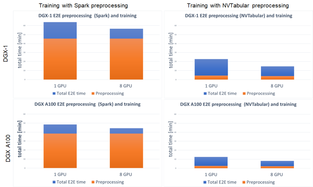
Four bar charts with the difference between preprocessing and preprocessing with model training, between one GPU and eight GPUs. — Figure 7. The comparison of end-to-end training (preprocessing with model training) for DGX-1 (1st row) and DGX A100 (2nd row) for Spark-CPU preprocessing and model training (1st column) and NVTabular GPU preprocessing. Orange bar accounts for preprocessing, blue one is the preprocessing with model training.

For both DGX-1 and DGX A100, the speedup in end-to-end training is tremendous. Because this setup involved training the model on GPU for both Spark and NVTabular, the speedup comes from the preprocessing steps. It results in up to 3.8x faster end-to-end training for DGX-1 and up to 5.4x for DGX A100. When using GPU for preprocessing the fraction, the important aspect is the decreased time that the preprocessing step takes in total end-to-end training, from ~75% for Spark GPU down to ~25% for NVTabular.

Summary

In this post, we demonstrated an end-to-end preprocessing and training pipeline for the Wide & Deep model. We showed you how to get at least a 10x reduction in dataset preprocessing time using GPU preprocessing with NVTabular. Such an incredible speedup enables you to quickly verify your hypotheses about the data and bring new features to production.

We also showed the stability of training while reaching the evaluation score of MAP@12 for multiple training setups:

NVIDIA Ampere Architecture
NVIDIA Volta Architecture
Multi-GPU training
AMP training
XLA

Thanks to the great speedup that these features provide, you can train on the 8-GB dataset in less than 25s/epoch. The model throughput compared to CPU is over 100x higher on GPU. Finally, we showed the evaluation throughput that achieves 21Mln [samples] from a model checkpoint.

Future work for the Wide & Deep TensorFlow 2 implementation will concentrate on inference in Triton Server, improving the data loader to support parquet input files, and upgrading preprocessing in NVTabular to a recently released API version.

We encourage you to check our implementation of the Wide & Deep model in the NVIDIA DeepLearningExamples GitHub repository. In the comments, please tell us how you plan to adopt and extend this project.