
|
submitted by /u/xusty [visit reddit] [comments] |

 DataBloom
|
|
submitted by /u/xusty [visit reddit] [comments] |


|
submitted by /u/AR_MR_XR [visit reddit] [comments] |
 Satinder Singh won the Jetson Project of the Month for DeepWay, an AI-based navigation assistance system for the visually impaired. The project, which runs on an NVIDIA Jetson Nano Developer Kit, monitors the path of a person and provides guidance to walk on the correct side and avoid any oncoming pedestrians. In addition to the … Continued
Satinder Singh won the Jetson Project of the Month for DeepWay, an AI-based navigation assistance system for the visually impaired. The project, which runs on an NVIDIA Jetson Nano Developer Kit, monitors the path of a person and provides guidance to walk on the correct side and avoid any oncoming pedestrians.
In addition to the Jetson Nano, Satinder’s setup includes an Arduino Nano, a webcam, two servo motors, a USB audio adapter, 3D printed eye-glasses and a few peripherals. The Arduino Nano is used to control the servo motors, which nudge the user in the correct direction by gently tapping them on either side of the head. If the Jetson Nano identifies pedestrians, a voice prompt sent through the USB audio adapter can be used to warn the user.
To train his convolutional neural network, Satinder collected 10,000 images across three classes for left, center and right positions within a lane, and trained his model on a GPU-enabled virtual machine on Microsoft Azure. He used both PyTorch and Keras for training a U-net semantic segmentation model. After further analysis, he picked the U-Net model trained in Keras for its better performance.
DeepWay – Project Walk Through
Satinder believes that his solution stands out among others because of its portability and affordability (plan including further optimizing it using NVIDIA TensorRT. We can’t wait to see how this project evolves.
The World Health Organization estimates at least 2.2 billion people around the world have a vision impairment. Many among this group would benefit from navigation aids. Open-source prototypes such as DeepWay foster innovation around these use-cases and are great examples of AI being used for social good.
If you’re interested in building your own ‘DeepWay’ or extending it, Satinder has shared the instructions and the code here.
When French classmates Guillaume Jourdain, Hugo Serrat and Jules Beguerie were looking at applying AI to agriculture in 2014 to form a startup, it was hardly a sure bet. It was early days for such AI applications, and people said it couldn’t be done. But farmers they spoke with wanted it. So they rigged together Read article >
The post Harvesting AI: Startup’s Weed Recognition for Herbicides Grows Yield for Farmers appeared first on The Official NVIDIA Blog.
Updated for TensorFlow 2
Google’s TensorFlow has been a hot topic in deep learning recently. The open source software, designed to allow efficient computation of data flow graphs, is especially suited to deep learning tasks. It is designed to be executed on single or multiple CPUs and GPUs, making it a good option for complex deep learning tasks. In its most recent incarnation – version 1.0 – it can even be run on certain mobile operating systems. This introductory tutorial to TensorFlow will give an overview of some of the basic concepts of TensorFlow in Python. These will be a good stepping stone to building more complex deep learning networks, such as Convolution Neural Networks, natural language models, and Recurrent Neural Networks in the package. We’ll be creating a simple three-layer neural network to classify the MNIST dataset. This tutorial assumes that you are familiar with the basics of neural networks, which you can get up to scratch with in the neural networks tutorial if required. To install TensorFlow, follow the instructions here. The code for this tutorial can be found in this site’s GitHub repository. Once you’re done, you also might want to check out a higher level deep learning library that sits on top of TensorFlow called Keras – see my Keras tutorial.
First, let’s have a look at the main ideas of TensorFlow.
1.0 TensorFlow graphs
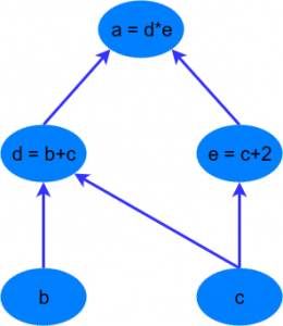
TensorFlow is based on graph based computation – “what on earth is that?”, you might say. It’s an alternative way of conceptualising mathematical calculations. Consider the following expression $a = (b + c) * (c + 2)$. We can break this function down into the following components:
begin{align}
d &= b + c \
e &= c + 2 \
a &= d * e
end{align}
Now we can represent these operations graphically as:

Simple computational graph
This may seem like a silly example – but notice a powerful idea in expressing the equation this way: two of the computations ($d=b+c$ and $e=c+2$) can be performed in parallel. By splitting up these calculations across CPUs or GPUs, this can give us significant gains in computational times. These gains are a must for big data applications and deep learning – especially for complicated neural network architectures such as Convolutional Neural Networks (CNNs) and Recurrent Neural Networks (RNNs). The idea behind TensorFlow is to the ability to create these computational graphs in code and allow significant performance improvements via parallel operations and other efficiency gains.
We can look at a similar graph in TensorFlow below, which shows the computational graph of a three-layer neural network.

TensorFlow data flow graph
The animated data flows between different nodes in the graph are tensors which are multi-dimensional data arrays. For instance, the input data tensor may be 5000 x 64 x 1, which represents a 64 node input layer with 5000 training samples. After the input layer, there is a hidden layer with rectified linear units as the activation function. There is a final output layer (called a “logit layer” in the above graph) that uses cross-entropy as a cost/loss function. At each point we see the relevant tensors flowing to the “Gradients” block which finally flows to the Stochastic Gradient Descent optimizer which performs the back-propagation and gradient descent.
Here we can see how computational graphs can be used to represent the calculations in neural networks, and this, of course, is what TensorFlow excels at. Let’s see how to perform some basic mathematical operations in TensorFlow to get a feel for how it all works.
2.0 A Simple TensorFlow example
So how can we make TensorFlow perform the little example calculation shown above – $a = (b + c) * (c + 2)$? First, there is a need to introduce TensorFlow variables. The code below shows how to declare these objects:
import tensorflow as tf
# create TensorFlow variables
const = tf.Variable(2.0, name="const")
b = tf.Variable(2.0, name='b')
c = tf.Variable(1.0, name='c')
As can be observed above, TensorFlow variables can be declared using the tf.Variable function. The first argument is the value to be assigned to the variable. The second is an optional name string which can be used to label the constant/variable – this is handy for when you want to do visualizations. TensorFlow will infer the type of the variable from the initialized value, but it can also be set explicitly using the optional dtype argument. TensorFlow has many of its own types like tf.float32, tf.int32 etc.
The objects assigned to the Python variables are actually TensorFlow tensors. Thereafter, they act like normal Python objects – therefore, if you want to access the tensors you need to keep track of the Python variables. In previous versions of TensorFlow, there were global methods of accessing the tensors and operations based on their names. This is no longer the case.
To examine the tensors stored in the Python variables, simply call them as you would a normal Python variable. If we do this for the “const” variable, you will see the following output:
<tf.Variable ‘const:0’ shape=() dtype=float32, numpy=2.0>
This output gives you a few different pieces of information – first, is the name ‘const:0’ which has been assigned to the tensor. Next is the data type, in this case, a TensorFlow float 32 type. Finally, there is a “numpy” value. TensorFlow variables in TensorFlow 2 can be converted easily into numpy objects. Numpy stands for Numerical Python and is a crucial library for Python data science and machine learning. If you don’t know Numpy, what it is, and how to use it, check out this site. The command to access the numpy form of the tensor is simply .numpy() – the use of this method will be shown shortly.
Next, some calculation operations are created:
# now create some operations
d = tf.add(b, c, name='d')
e = tf.add(c, const, name='e')
a = tf.multiply(d, e, name='a')
Note that d and e are automatically converted to tensor values upon the execution of the operations. TensorFlow has a wealth of calculation operations available to perform all sorts of interactions between tensors, as you will discover as you progress through this book. The purpose of the operations shown above are pretty obvious, and they instantiate the operations b + c, c + 2.0, and d * e. However, these operations are an unwieldy way of doing things in TensorFlow 2. The operations below are equivalent to those above:
d = b + c
e = c + 2
a = d * e
To access the value of variable a, one can use the .numpy() method as shown below:
print(f”Variable a is {a.numpy()}”)
The computational graph for this simple example can be visualized by using the TensorBoard functionality that comes packaged with TensorFlow. This is a great visualization feature and is explained more in this post. Here is what the graph looks like in TensorBoard:

Simple TensorFlow graph
The larger two vertices or nodes, b and c, correspond to the variables. The smaller nodes correspond to the operations, and the edges between the vertices are the scalar values emerging from the variables and operations.
The example above is a trivial example – what would this look like if there was an array of b values from which an array of equivalent a values would be calculated? TensorFlow variables can easily be instantiated using numpy variables, like the following:
b = tf.Variable(np.arange(0, 10), name='b')
Calling b shows the following:
<tf.Variable ‘b:0’ shape=(10,) dtype=int32, numpy=array([0, 1, 2, 3, 4, 5, 6, 7, 8, 9])>
Note the numpy value of the tensor is an array. Because the numpy variable passed during the instantiation is a range of int32 values, we can’t add it directly to c as c is of float32 type. Therefore, the tf.cast operation, which changes the type of a tensor, first needs to be utilized like so:
d = tf.cast(b, tf.float32) + c
Running the rest of the previous operations, using the new b tensor, gives the following value for a:
Variable a is [ 3. 6. 9. 12. 15. 18. 21. 24. 27. 30.]
In numpy, the developer can directly access slices or individual indices of an array and change their values directly. Can the same be done in TensorFlow 2? Can individual indices and/or slices be accessed and changed? The answer is yes, but not quite as straight-forwardly as in numpy. For instance, if b was a simple numpy array, one could easily execute the following b[1] = 10 – this would change the value of the second element in the array to the integer 10.
b[1].assign(10)
This will then flow through to a like so:
Variable a is [ 3. 33. 9. 12. 15. 18. 21. 24. 27. 30.]
The developer could also run the following, to assign a slice of b values:
b[6:9].assign([10, 10, 10])
A new tensor can also be created by using the slice notation:
f = b[2:5]
The explanations and code above show you how to perform some basic tensor manipulations and operations. In the section below, an example will be presented where a neural network is created using the Eager paradigm in TensorFlow 2. It will show how to create a training loop, perform a feed-forward pass through a neural network and calculate and apply gradients to an optimization method.
3.0 A Neural Network Example
In this section, a simple three-layer neural network build in TensorFlow is demonstrated. In following chapters more complicated neural network structures such as convolution neural networks and recurrent neural networks are covered. For this example, though, it will be kept simple.
In this example, the MNIST dataset will be used that is packaged as part of the TensorFlow installation. This MNIST dataset is a set of 28×28 pixel grayscale images which represent hand-written digits. It has 60,000 training rows, 10,000 testing rows, and 5,000 validation rows. It is a very common, basic, image classification dataset that is used in machine learning.
The data can be loaded by running the following:
from tensorflow.keras.datasets import mnist
(x_train, y_train), (x_test, y_test) = mnist.load_data()
As can be observed, the Keras MNIST data loader returns Python tuples corresponding to the training and test set respectively (Keras is another deep learning framework, now tightly integrated with TensorFlow, as mentioned earlier). The data sizes of the tuples defined above are:
The x data is the image information – 60,000 images of 28 x 28 pixels size in the training set. The images are grayscale (i.e black and white) with maximum values, specifying the intensity of whites, of 255. The x data will need to be scaled so that it resides between 0 and 1, as this improves training efficiency. The y data is the matching image labels – signifying what digit is displayed in the image. This will need to be transformed to “one-hot” format.
When using a standard, categorical cross-entropy loss function (this will be shown later), a one-hot format is required when training classification tasks, as the output layer of the neural network will have the same number of nodes as the total number of possible classification labels. The output node with the highest value is considered as a prediction for that corresponding label. For instance, in the MNIST task, there are 10 possible classification labels – 0 to 9. Therefore, there will be 10 output nodes in any neural network performing this classification task. If we have an example output vector of [0.01, 0.8, 0.25, 0.05, 0.10, 0.27, 0.55, 0.32, 0.11, 0.09], the maximum value is in the second position / output node, and therefore this corresponds to the digit “1”. To train the network to produce this sort of outcome when the digit “1” appears, the loss needs to be calculated according to the difference between the output of the network and a “one-hot” array of the label 1. This one-hot array looks like [0, 1, 0, 0, 0, 0, 0, 0, 0, 0].
This conversion is easily performed in TensorFlow, as will be demonstrated shortly when the main training loop is covered.
One final thing that needs to be considered is how to extract the training data in batches of samples. The function below can handle this:
def get_batch(x_data, y_data, batch_size):
    idxs = np.random.randint(0, len(y_data), batch_size)
    return x_data[idxs,:,:], y_data[idxs]
As can be observed in the code above, the data to be batched i.e. the x and y data is passed to this function along with the batch size. The first line of the function generates a random vector of integers, with random values between 0 and the length of the data passed to the function. The number of random integers generated is equal to the batch size. The x and y data are then returned, but the return data is only for those random indices chosen. Note, that this is performed on numpy array objects – as will be shown shortly, the conversion from numpy arrays to tensor objects will be performed “on the fly” within the training loop.
There is also the requirement for a loss function and a feed-forward function, but these will be covered shortly.
# Python optimisation variables
epochs = 10
batch_size = 100

# normalize the input images by dividing by 255.0
x_train = x_train / 255.0
x_test = x_test / 255.0
# convert x_test to tensor to pass through model (train data will be converted to
# tensors on the fly)
x_test = tf.Variable(x_test)
First, the number of training epochs and the batch size are created – note these are simple Python variables, not TensorFlow variables. Next, the input training and test data, x_train and x_test, are scaled so that their values are between 0 and 1. Input data should always be scaled when training neural networks, as large, uncontrolled, inputs can heavily impact the training process. Finally, the test input data, x_test is converted into a tensor. The random batching process for the training data is most easily performed using numpy objects and functions. However, the test data will not be batched in this example, so the full test input data set x_test is converted into a tensor.
The next step is to setup the weight and bias variables for the three-layer neural network. There are always L – 1 number of weights/bias tensors, where L is the number of layers. These variables are defined in the code below:
# now declare the weights connecting the input to the hidden layer
W1 = tf.Variable(tf.random.normal([784, 300], stddev=0.03), name='W1')
b1 = tf.Variable(tf.random.normal([300]), name='b1')
# and the weights connecting the hidden layer to the output layer
W2 = tf.Variable(tf.random.normal([300, 10], stddev=0.03), name='W2')
b2 = tf.Variable(tf.random.normal([10]), name='b2')
The weight and bias variables are initialized using the tf.random.normal function – this function creates tensors of random numbers, drawn from a normal distribution. It allows the developer to specify things like the standard deviation of the distribution from which the random numbers are drawn.
Note the shape of the variables. The W1 variable is a [784, 300] tensor – the 784 nodes are the size of the input layer. This size comes from the flattening of the input images – if we have 28 rows and 28 columns of pixels, flattening these out gives us 1 row or column of 28 x 28 = 784 values. The 300 in the declaration of W1 is the number of nodes in the hidden layer. The W2 variable is a [300, 10] tensor, connecting the 300-node hidden layer to the 10-node output layer. In each case, a name is given to the variable for later viewing in TensorBoard – the TensorFlow visualization package. The next step in the code is to create the computations that occur within the nodes of the network. If the reader recalls, the computations within the nodes of a neural network are of the following form:
$$z = Wx + b$$
$$h=f(z)$$
Where W is the weights matrix, x is the layer input vector, b is the bias and f is the activation function of the node. These calculations comprise the feed-forward pass of the input data through the neural network. To execute these calculations, a dedicated feed-forward function is created:
def nn_model(x_input, W1, b1, W2, b2):
    # flatten the input image from 28 x 28 to 784
    x_input = tf.reshape(x_input, (x_input.shape[0], -1))
    x = tf.add(tf.matmul(tf.cast(x_input, tf.float32), W1), b1)
    x = tf.nn.relu(x)
    logits = tf.add(tf.matmul(x, W2), b2)
    return logits
Examining the first line, the x_input data is reshaped from (batch_size, 28, 28) to (batch_size, 784) – in other words, the images are flattened out. On the next line, the input data is then converted to tf.float32 type using the TensorFlow cast function. This is important – the x_input data comes in as tf.float64 type, and TensorFlow won’t perform a matrix multiplication operation (tf.matmul) between tensors of different data types. This re-typed input data is then matrix-multiplied by W1 using the TensorFlow matmul function (which stands for matrix multiplication). Then the bias b1 is added to this product. On the line after this, the ReLU activation function is applied to the output of this line of calculation. The ReLU function is usually the best activation function to use in deep learning – the reasons for this are discussed in this post.
The output of this calculation is then multiplied by the final set of weights W2, with the bias b2 added. The output of this calculation is titled logits. Note that no activation function has been applied to this output layer of nodes (yet). In machine/deep learning, the term “logits” refers to the un-activated output of a layer of nodes.
The reason no activation function has been applied to this layer is that there is a handy function in TensorFlow called tf.nn.softmax_cross_entropy_with_logits. This function does two things for the developer – it applies a softmax activation function to the logits, which transforms them into a quasi-probability (i.e. the sum of the output nodes is equal to 1). This is a common activation function to apply to an output layer in classification tasks. Next, it applies the cross-entropy loss function to the softmax activation output. The cross-entropy loss function is a commonly used loss in classification tasks. The theory behind it is quite interesting, but it won’t be covered in this book – a good summary can be found here. The code below applies this handy TensorFlow function, and in this example, it has been nested in another function called loss_fn:
def loss_fn(logits, labels):
    cross_entropy = tf.reduce_mean(tf.nn.softmax_cross_entropy_with_logits(labels=labels,
                                                                              logits=logits))
    return cross_entropy
The arguments to softmax_cross_entropy_with_logits are labels and logits. The logits argument is supplied from the outcome of the nn_model function. The usage of this function in the main training loop will be demonstrated shortly. The labels argument is supplied from the one-hot y values that are fed into loss_fn during the training process. The output of the softmax_cross_entropy_with_logits function will be the output of the cross-entropy loss value for each sample in the batch. To train the weights of the neural network, the average cross-entropy loss across the samples needs to be minimized as part of the optimization process. This is calculated by using the tf.reduce_mean function, which, unsurprisingly, calculates the mean of the tensor supplied to it.
The next step is to define an optimizer function. In many examples within this book, the versatile Adam optimizer will be used. The theory behind this optimizer is interesting, and is worth further examination (such as shown here) but won’t be covered in detail within this post. It is basically a gradient descent method, but with sophisticated averaging of the gradients to provide appropriate momentum to the learning. To define the optimizer, which will be used in the main training loop, the following code is run:
# setup the optimizer
optimizer = tf.keras.optimizers.Adam()
The Adam object can take a learning rate as input, but for the present purposes, the default value is used.
3.1 Training the network
Now that the appropriate functions, variables and optimizers have been created, it is time to define the overall training loop. The training loop is shown below:
total_batch = int(len(y_train) / batch_size)
for epoch in range(epochs):
    avg_loss = 0
    for i in range(total_batch):
        batch_x, batch_y = get_batch(x_train, y_train, batch_size=batch_size)
        # create tensors
        batch_x = tf.Variable(batch_x)
        batch_y = tf.Variable(batch_y)
        # create a one hot vector
        batch_y = tf.one_hot(batch_y, 10)
        with tf.GradientTape() as tape:
            logits = nn_model(batch_x, W1, b1, W2, b2)
            loss = loss_fn(logits, batch_y)
        gradients = tape.gradient(loss, [W1, b1, W2, b2])
        optimizer.apply_gradients(zip(gradients, [W1, b1, W2, b2]))
        avg_loss += loss /..
In a previous post, I gave an introduction to Policy Gradient reinforcement learning. Policy gradient-based reinforcement learning relies on using neural networks to learn an action policy for the control of agents in an environment. This is opposed to controlling agents based on neural network estimations of a value-based function, such as the Q value in deep Q learning. However, there are problems with straight Monte-Carlo based methods of policy gradient learning as covered in the previously mentioned policy gradient post. In particular, one significant problem is a high variance in the learning. This problem can be solved by a process called baselining, with the most effective baselining method being the Advantage Actor Critic method or A2c. In this post, I’ll review the theory of the A2c method, and demonstrate how to build an A2c algorithm in TensorFlow 2.
All code shown in this tutorial can be found at this site’s Github repository, in the ac2_tf2_cartpole.py file.
A quick recap of some important concepts
In the A2C algorithm, notice the title “Advantage Actor” – this refers first to the actor, the part of the neural network that is used to determine the actions of the agent. The “advantage” is a concept that expresses the relative benefit of taking a certain action at time t ($a_t$) from a certain state $s_t$. Note that it is not the “absolute” benefit, but the “relative” benefit. This will become clearer when I discuss the concept of “value”. The advantage is expressed as:
$$A(s_t, a_t) = Q(s_t, a_t) – V(s_t)$$
The Q value (discussed in other posts, for instance here, here and here) is the expected future rewards of taking action $a_t$ from state $s_t$. The value $V(s_t)$ is the expected value of the agent being in that state and operating under a certain action policy $pi$. It can be expressed as:
$$V^{pi}(s) = mathbb{E} left[sum_{i=1}^T gamma^{i-1}r_{i}right]$$
Here $mathbb{E}$ is the expectation operator, and the value $V^{pi}(s)$ can be read as the expected value of future discounted rewards that will be gathered by the agent, operating under a certain action policy $pi$. So, the Q value is the expected value of taking a certain action from the current state, whereas V is the expected value of simply being in the current state, under a certain action policy.
The advantage then is the relative benefit of taking a certain action from the current state. It’s kind of like a normalized Q value. For example, let’s consider the last state in a game, where after the next action the game ends. There are three possible actions from this state, with rewards of (51, 50, 49). Let’s also assume that the action selection policy $pi$ is simply random, so there is an equal chance of any of the three actions being selected. The value of this state, then, is 50 ((51+50+49) / 3). If the first action is randomly selected (reward=51), the Q value is 51. However, the advantage is only equal to 1 (Q-V = 51-50). As can be observed and as stated above, the advantage is a kind of normalized or relative Q value.
Why is this important? If we are using Q values in some way to train our action-taking policy, in the example above the first action would send a “signal” or contribution of 51 to the gradient optimizer, which may be significant enough to push the parameters of the neural network significantly in a certain direction. However, given the other two actions possible from this state also have a high reward (50 and 49), the signal or contribution is really higher than it should be – it is not that much better to take action 1 instead of action 3. Therefore, Q values can be a source of high variance in the training process, and it is much better to use the normalized or baseline Q values i.e. the advantage, in training. For more discussion of Q, values, and advantages, see my post on dueling Q networks.
Policy gradient reinforcement learning and its problems
In a previous post, I presented the policy gradient reinforcement learning algorithm. For details on this algorithm, please consult that post. However, the A2C algorithm shares important similarities with the PG algorithm, and therefore it is necessary to recap some of the theory. First, it has to be recalled that PG-based algorithms involve a neural network that directly outputs estimates of the probability distribution of the best next action to take in a given state. So, for instance, if we have an environment with 4 possible actions, the output from the neural network could be something like [0.5, 0.25, 0.1, 0.15], with the first action being currently favored. In the PG case, then, the neural network is the direct instantiation of the policy of the agent $pi_{theta}$ – where this policy is controlled by the parameters of the neural network $theta$. This is opposed to Q based RL algorithms, where the neural network estimates the Q value in a given state for each possible action. In these algorithms, the action policy is generally an epsilon-greedy policy, where the best action is that action with the highest Q value (with some random choices involved to improve exploration).
The gradient of the loss function for the policy gradient algorithm is as follows:
$$nabla_theta J(theta) sim left(sum_{t=0}^{T-1} log P_{pi_{theta}}(a_t|s_t)right)left(sum_{t’= t + 1}^{T} gamma^{t’-t-1} r_{t’} right)$$
Note that the term:
$$G_t = left(sum_{t’= t + 1}^{T} gamma^{t’-t-1} r_{t’} right)$$
Is just the discounted sum of the rewards onwards from state $s_t$. In other words, it is an estimate of the true value function $V^{pi}(s)$. Remember that in the PG algorithm, the network can only be trained after each full episode, and this is because of the term above. Therefore, note that the $G_t$ term above is an estimate of the true value function as it is based on only a single trajectory of the agent through the game.
Now, because it is based on samples of reward trajectories, which aren’t “normalized” or baselined in any way, the PG algorithm suffers from variance issues, resulting in slower and more erratic training progress. A better solution is to replace the $G_t$ function above with the Advantage – $A(s_t, a_t)$, and this is what the Advantage-Actor Critic method does.
The A2C algorithm
Replacing the $G_t$ function with the advantage, we come up with the following gradient function which can be used in training the neural network:
$$nabla_theta J(theta) sim left(sum_{t=0}^{T-1} log P_{pi_{theta}}(a_t|s_t)right)A(s_t, a_t)$$
Now, as shown above, the advantage is:
$$A(s_t, a_t) = Q(s_t, a_t) – V(s_t)$$
However, using Bellman’s equation, the Q value can be expressed purely in terms of the rewards and the value function:
$$Q(s_t, a_t) = mathbb{E}left[r_{t+1} + gamma V(s_{t+1})right]$$
Therefore, the advantage can now be estimated as:
$$A(s_t, a_t) = r_{t+1} + gamma V(s_{t+1}) – V(s_t)$$
As can be seen from the above, there is a requirement to be able to estimate the value function V. We could estimate it by running our agents through full episodes, in the same way we did in the policy gradient method. However, it would be better to be able to just collect batches of game-steps and train whenever the batch buffer was full, rather than having to wait for an episode to finish. That way, the agent could actually learn “on-the-go” during the middle of an episode/game.
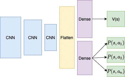
So, do we build another neural network to estimate V? We could have two networks, one to learn the policy and produce actions, and another to estimate the state values. A more efficient solution is to create one network, but with two output channels, and this is how the A2C method is outworked. The figure below shows the network architecture for an A2C neural network:

A2C architecture
This architecture is based on an A2C method that takes game images as the state input, hence the convolutional neural network layers at the beginning of the network (for more on CNNs, see my post here). This network architecture also resembles the Dueling Q network architecture (see my Dueling Q post). The point to note about the architecture above is that most of the network is shared, with a late bifurcation between the policy part and the value part. The outputs $P(s, a_i)$ are the action probabilities of the policy (generated from the neural network) – $P(a_t|s_t)$. The other output channel is the value estimation – a scalar output which is the predicted value of state s – $V(s)$. The two dense channels disambiguate the policy and the value outputs from the front-end of the neural network.
In this example, we’ll just be demonstrating the A2C algorithm on the Cartpole OpenAI Gym environment which doesn’t require a visual state input (i.e. a set of pixels as the input to the NN), and therefore the two output channels will simply share some dense layers, rather than a series of CNN layers.
The A2C loss functions
There are actually three loss values that need to be calculated in the A2C algorithm. Each of these losses is in practice given a weighting, and then they are summed together (with the entropy loss having a negative sign, see below).
The Critic loss
The loss function of the Critic i.e. the value estimating output of the neural network $V(s)$, needs to be trained so that it predicts more and more closely the actual value of the state. As shown before, the value of a state is calculated as:
$$V^{pi}(s) = mathbb{E} left[sum_{i=1}^T gamma^{i-1}r_{i}right]$$
So $V^{pi}(s)$ is the expected value of the discounted future rewards obtained by outworking a trajectory through the game based on a certain operating policy $pi$. We can therefore compare the predicted $V(s)$ at each state in the game, and the actual sampled discounted rewards that were gathered, and the difference between the two is the Critic loss. In this example, we’ll use a mean squared error function as the loss function, between the discounted rewards and the predicted values ($(V(s) – DR)^2$).
Now, given that, under the A2C algorithm, we collect state, action and reward tuples until a batch buffer is filled, how are we meant to figure out this discounted rewards sum? Let’s say we progress 3 states through a game, and we collect:
$(V(s_0), r_0), (V(s_1), r_1), (V(s_2), r_2)$
For the first Critic loss, we could calculate it as:
$$MSE(V(s_0), r_0 + gamma r_1 + gamma^2 r_2)$$
But that is missing all the following rewards $r_3, r_4, …., r_n$ until the game terminates. We didn’t have this problem in the Policy Gradient method, because in that method, we made sure a full run through the game had completed before training the neural network. In the A2c method, we use a trick called bootstrapping. To replace all the discounted $r_3, r_4, …., r_n$ values, we get the network to estimate the value for state 3, $V(s_3)$, and this will be an estimate for all the discounted future rewards beyond that point in the game. So, for the first Critic loss, we would have:
$$MSE(V(s_0), r_0 + gamma r_1 + gamma^2 r_2 + gamma^3 V(s_3))$$
Where $V(s_3)$ is a bootstrapped estimate of the value of the next state $s_3$.
This will be explained more in the code-walkthrough to follow.
The Actor loss
The second loss function needs to train the Actor (i.e. the action policy). Recall that the advantage weighted policy loss is:
$$nabla_theta J(theta) sim left(sum_{t=0}^{T-1} log P_{pi_{theta}}(a_t|s_t)right)A(s_t, a_t)$$
Let’s start with the advantage – $A(s_t, a_t) = r_{t+1} + gamma V(s_{t+1}) – V(s_t)$
This is simply the bootstrapped discounted rewards minus the predicted state values $V(s_t)$ that we gathered up while playing the game. So calculating the advantage is quite straight-forward, once we have the bootstrapped discounted rewards, as will be seen in the code walk-through shortly.
Now, with regards to the $log P_{pi_{theta}}(a_t|s_t)$ statement, in this instance, we can just calculate the log of the softmax probability estimate for whatever action was taken. So, for instance, if in state 1 ($s_1$) the network softmax output produces {0.1, 0.9} (for a 2-action environment), and the second action was actually taken by the agent, we would want to calculate log(0.9). We can make use of the TensorFlow-Keras SparseCategoricalCrossEntropy calculation, which takes the action as an integer, and this specifies which softmax output value to apply the log to. So in this example, y_pred = [1] and y_target = [0.1, 0.9] and the answer would be -log(0.9) = 0.105.
Another handy feature with the SpareCategoricalCrossEntropy loss in Keras is that it can be called with a “sample_weight” argument. This basically multiplies the log calculation with a value. So, in this example, we can supply the advantages as the sample weights, and it will calculate $nabla_theta J(theta) sim left(sum_{t=0}^{T-1} log P_{pi_{theta}}(a_t|s_t)right)A(s_t, a_t)$ for us. This will be shown below, but the call will look like:
policy_loss = sparse_ce(actions, policy_logits, sample_weight=advantages)
Entropy loss
In many implementations of the A2c algorithm, another loss term is subtracted – the entropy loss. Entropy is a measure, broadly speaking, of randomness. The higher the entropy, the more random the state of affairs, the lower the entropy, the more ordered the state of affairs. In the case of A2c, entropy is calculated on the softmax policy action ($P(a_t|s_t)$) output of the neural network. Let’s go back to our two action example from above. In the case of a probability output of {0.1, 0.9} for the two possible actions, this is an ordered, less-random selection of actions. In other words, there will be a consistent selection of action 2, and only rarely will action 1 be taken. The entropy formula is:
$$E = -sum p(x) log(p(x))$$
So in this case, the entropy of that output would be 0.325. However, if the probability output was instead {0.5, 0.5}, the entropy would be 0.693. The 50-50 action probability distribution will produce more random actions, and therefore the entropy is higher.
By subtracting the entropy calculation from the total loss (or giving the entropy loss a negative sign), it encourages more randomness and therefore more exploration. The A2c algorithm can have a tendency of converging on particular actions, so this subtraction of the entropy encourages a better exploration of alternative actions, though making the weighting on this component of the loss too large can also reduce training performance.
Again, we can use an already existing Keras loss function to calculate the entropy. The Keras categorical cross-entropy performs the following calculation:
Keras output of cross-entropy loss function
If we just pass in the probability outputs as both target and output to this function, then it will calculate the entropy for us. This will be shown in the code below.
The total loss
The total loss function for the A2C algorithm is:
Loss = Actor Loss + Critic Loss * CRITIC_WEIGHT – Entropy Loss * ENTROPY_WEIGHT
A common value for the critic weight is 0.5, and the entropy weight is usually quite low (i.e. on the order of 0.01-0.001), though these hyperparameters can be adjusted and experimented with depending on the environment and network.
Implementing A2C in TensorFlow 2
In the following section, I will provide a walk-through of some code to implement the A2C methodology in TensorFlow 2. The code for this can be found at this site’s Github repository, in the ac2_tf2_cartpole.py file.
First, we perform the usual imports, set some constants, initialize the environment and finally create the neural network model which instantiates the A2C architecture:
import tensorflow as tf
from tensorflow import keras
import numpy as np
import gym
import datetime as dt

STORE_PATH = '/Users/andrewthomas/Adventures in ML/TensorFlowBook/TensorBoard/A2CCartPole'
CRITIC_LOSS_WEIGHT = 0.5
ACTOR_LOSS_WEIGHT = 1.0
ENTROPY_LOSS_WEIGHT = 0.05
BATCH_SIZE = 64
GAMMA = 0.95

env = gym.make("CartPole-v0")
state_size = 4
num_actions = env.action_space.n


class Model(keras.Model):
    def __init__(self, num_actions):
        super().__init__()
        self.num_actions = num_actions
        self.dense1 = keras.layers.Dense(64, activation='relu',
                                         kernel_initializer=keras.initializers.he_normal())
        self.dense2 = keras.layers.Dense(64, activation='relu',
                                         kernel_initializer=keras.initializers.he_normal())
        self.value = keras.layers.Dense(1)
        self.policy_logits = keras.layers.Dense(num_actions)

    def call(self, inputs):
        x = self.dense1(inputs)
        x = self.dense2(x)
        return self.value(x), self.policy_logits(x)

    def action_value(self, state):
        value, logits = self.predict_on_batch(state)
        action = tf.random.categorical(logits, 1)[0]
        return action, value
As can be seen, for this example I have set the critic, actor and entropy loss weights to 0.5, 1.0 and 0.05 respectively. Next the environment is setup, and then the model class is created.
This class inherits from keras.Model, which enables it to be integrated into the streamlined Keras methods of training and evaluating (for more information, see this Keras tutorial). In the initialization of the class, we see that 2 dense layers have been created, with 64 nodes in each. Then a value layer with one output is created, which evaluates $V(s)$, and finally the policy layer output with a size equal to the number of available actions. Note that this layer produces logits only, the softmax function which creates pseudo-probabilities ($P(a_t, s_t)$) will be applied within the various TensorFlow functions, as will be seen.
Next, the call function is defined – this function is run whenever a state needs to be “run” through the model, to produce a value and policy logits output. The Keras model API will use this function in its predict functions and also its training functions. In this function, it can be observed that the input is passed through the two common dense layers, and then the function returns first the value output, then the policy logits output.
The next function is the action_value function. This function is called upon when an action needs to be chosen from the model. As can be seen, the first step of the function is to run the predict_on_batch Keras model API function. This function just runs the model.call function defined above. The output is both the values and the policy logits. An action is then selected by randomly choosing an action based on the action probabilities. Note that tf.random.categorical takes as input logits, not softmax outputs. The next function, outside of the Model class, is the function that calculates the critic loss:
def critic_loss(discounted_rewards, predicted_values):
    return keras.losses.mean_squared_error(discounted_rewards, predicted_values) * CRITIC_LOSS_WEIGHT
As explained above, the critic loss comprises of the mean squared error between the discounted rewards (which is calculated in another function, soon to be discussed) and the values predicted from the value output of the model (which are accumulated in a list during the agent’s trajectory through the game).
The following function shows the actor loss function:
def actor_loss(combined, policy_logits):
    actions = combined[:, 0]
    advantages = combined[:, 1]
    sparse_ce = keras.losses.SparseCategoricalCrossentropy(
        from_logits=True, reduction=tf.keras.losses.Reduction.SUM
    )

    actions = tf.cast(actions, tf.int32)
    policy_loss = sparse_ce(actions, policy_logits, sample_weight=advantages)

    probs = tf.nn.softmax(policy_logits)
    entropy_loss = keras.losses.categorical_crossentropy(probs, probs)

    return policy_loss * ACTOR_LOSS_WEIGHT - entropy_loss * ENTROPY_LOSS_WEIGHT
The first argument to the actor_loss function is an array with two columns (and BATCH_SIZE rows). The first column corresponds to the recorded actions of the agent as it traversed the game. The second column is the calculated advantages – the calculation of which will be shown shortly. Next, the sparse categorical cross-entropy function class is created. The arguments specify that the input to the function is logits (i.e. they don’t have softmax applied to them yet), and it also specifies the reduction to apply to the BATCH_SIZE number of calculated losses – in this case, a sum() function which aligns with the summation in:
$$nabla_theta J(theta) sim left(sum_{t=0}^{T-1} log P_{pi_{theta}}(a_t|s_t)right)A(s_t, a_t)$$
Next, the actions are cast to be integers (rather than floats) and finally, the policy loss is calculated based on the sparse_ce function. As discussed above, the sparse categorical cross-entropy function will select those policy probabilities that correspond to the actions actually taken in the game, and weight them by the advantage values. By applying a summation reduction, the formula above will be implemented in this function.
Next, the actual probabilities for action are estimated by applying the softmax function to the logits, and the entropy loss is calculated by applying the categorical cross-entropy function. See the previous discussion on how this works.
The following function calculates the discounted reward values and the advantages:
def discounted_rewards_advantages(rewards, dones, values, next_value):
    discounted_rewards = np.array(rewards + [next_value[0]])

    for t in reversed(range(len(rewards))):
        discounted_rewards[t] = rewards[t] + GAMMA * discounted_rewards[t+1] * (1-dones[t])
    discounted_rewards = discounted_rewards[:-1]
    # advantages are bootstrapped discounted rewards - values, using Bellman's equation
    advantages = discounted_rewards - np.stack(values)[:, 0]
    return discounted_rewards, advantages
The first input value to this function is a list of all the rewards that were accumulated..
Updated for TensorFlow 2
Google’s TensorFlow has been a hot topic in deep learning recently. The open source software, designed to allow efficient computation of data flow graphs, is especially suited to deep learning tasks. It is designed to be executed on single or multiple CPUs and GPUs, making it a good option for complex deep learning tasks. In its most recent incarnation – version 1.0 – it can even be run on certain mobile operating systems. This introductory tutorial to TensorFlow will give an overview of some of the basic concepts of TensorFlow in Python. These will be a good stepping stone to building more complex deep learning networks, such as Convolution Neural Networks, natural language models, and Recurrent Neural Networks in the package. We’ll be creating a simple three-layer neural network to classify the MNIST dataset. This tutorial assumes that you are familiar with the basics of neural networks, which you can get up to scratch with in the neural networks tutorial if required. To install TensorFlow, follow the instructions here. The code for this tutorial can be found in this site’s GitHub repository. Once you’re done, you also might want to check out a higher level deep learning library that sits on top of TensorFlow called Keras – see my Keras tutorial.
First, let’s have a look at the main ideas of TensorFlow.
1.0 TensorFlow graphs
TensorFlow is based on graph based computation – “what on earth is that?”, you might say. It’s an alternative way of conceptualising mathematical calculations. Consider the following expression $a = (b + c) * (c + 2)$. We can break this function down into the following components:
begin{align}
d &= b + c \
e &= c + 2 \
a &= d * e
end{align}
Now we can represent these operations graphically as:
Simple computational graph
This may seem like a silly example – but notice a powerful idea in expressing the equation this way: two of the computations ($d=b+c$ and $e=c+2$) can be performed in parallel. By splitting up these calculations across CPUs or GPUs, this can give us significant gains in computational times. These gains are a must for big data applications and deep learning – especially for complicated neural network architectures such as Convolutional Neural Networks (CNNs) and Recurrent Neural Networks (RNNs). The idea behind TensorFlow is to the ability to create these computational graphs in code and allow significant performance improvements via parallel operations and other efficiency gains.
We can look at a similar graph in TensorFlow below, which shows the computational graph of a three-layer neural network.
TensorFlow data flow graph
The animated data flows between different nodes in the graph are tensors which are multi-dimensional data arrays. For instance, the input data tensor may be 5000 x 64 x 1, which represents a 64 node input layer with 5000 training samples. After the input layer, there is a hidden layer with rectified linear units as the activation function. There is a final output layer (called a “logit layer” in the above graph) that uses cross-entropy as a cost/loss function. At each point we see the relevant tensors flowing to the “Gradients” block which finally flows to the Stochastic Gradient Descent optimizer which performs the back-propagation and gradient descent.
Here we can see how computational graphs can be used to represent the calculations in neural networks, and this, of course, is what TensorFlow excels at. Let’s see how to perform some basic mathematical operations in TensorFlow to get a feel for how it all works.
2.0 A Simple TensorFlow example
So how can we make TensorFlow perform the little example calculation shown above – $a = (b + c) * (c + 2)$? First, there is a need to introduce TensorFlow variables. The code below shows how to declare these objects:
import tensorflow as tf
# create TensorFlow variables
const = tf.Variable(2.0, name="const")
b = tf.Variable(2.0, name='b')
c = tf.Variable(1.0, name='c')
As can be observed above, TensorFlow variables can be declared using the tf.Variable function. The first argument is the value to be assigned to the variable. The second is an optional name string which can be used to label the constant/variable – this is handy for when you want to do visualizations. TensorFlow will infer the type of the variable from the initialized value, but it can also be set explicitly using the optional dtype argument. TensorFlow has many of its own types like tf.float32, tf.int32 etc.
The objects assigned to the Python variables are actually TensorFlow tensors. Thereafter, they act like normal Python objects – therefore, if you want to access the tensors you need to keep track of the Python variables. In previous versions of TensorFlow, there were global methods of accessing the tensors and operations based on their names. This is no longer the case.
To examine the tensors stored in the Python variables, simply call them as you would a normal Python variable. If we do this for the “const” variable, you will see the following output:
<tf.Variable ‘const:0’ shape=() dtype=float32, numpy=2.0>
This output gives you a few different pieces of information – first, is the name ‘const:0’ which has been assigned to the tensor. Next is the data type, in this case, a TensorFlow float 32 type. Finally, there is a “numpy” value. TensorFlow variables in TensorFlow 2 can be converted easily into numpy objects. Numpy stands for Numerical Python and is a crucial library for Python data science and machine learning. If you don’t know Numpy, what it is, and how to use it, check out this site. The command to access the numpy form of the tensor is simply .numpy() – the use of this method will be shown shortly.
Next, some calculation operations are created:
# now create some operations
d = tf.add(b, c, name='d')
e = tf.add(c, const, name='e')
a = tf.multiply(d, e, name='a')
Note that d and e are automatically converted to tensor values upon the execution of the operations. TensorFlow has a wealth of calculation operations available to perform all sorts of interactions between tensors, as you will discover as you progress through this book. The purpose of the operations shown above are pretty obvious, and they instantiate the operations b + c, c + 2.0, and d * e. However, these operations are an unwieldy way of doing things in TensorFlow 2. The operations below are equivalent to those above:
d = b + c
e = c + 2
a = d * e
To access the value of variable a, one can use the .numpy() method as shown below:
print(f”Variable a is {a.numpy()}”)
The computational graph for this simple example can be visualized by using the TensorBoard functionality that comes packaged with TensorFlow. This is a great visualization feature and is explained more in this post. Here is what the graph looks like in TensorBoard:
Simple TensorFlow graph
The larger two vertices or nodes, b and c, correspond to the variables. The smaller nodes correspond to the operations, and the edges between the vertices are the scalar values emerging from the variables and operations.
The example above is a trivial example – what would this look like if there was an array of b values from which an array of equivalent a values would be calculated? TensorFlow variables can easily be instantiated using numpy variables, like the following:
b = tf.Variable(np.arange(0, 10), name='b')
Calling b shows the following:
<tf.Variable ‘b:0’ shape=(10,) dtype=int32, numpy=array([0, 1, 2, 3, 4, 5, 6, 7, 8, 9])>
Note the numpy value of the tensor is an array. Because the numpy variable passed during the instantiation is a range of int32 values, we can’t add it directly to c as c is of float32 type. Therefore, the tf.cast operation, which changes the type of a tensor, first needs to be utilized like so:
d = tf.cast(b, tf.float32) + c
Running the rest of the previous operations, using the new b tensor, gives the following value for a:
Variable a is [ 3. 6. 9. 12. 15. 18. 21. 24. 27. 30.]
In numpy, the developer can directly access slices or individual indices of an array and change their values directly. Can the same be done in TensorFlow 2? Can individual indices and/or slices be accessed and changed? The answer is yes, but not quite as straight-forwardly as in numpy. For instance, if b was a simple numpy array, one could easily execute the following b[1] = 10 – this would change the value of the second element in the array to the integer 10.
b[1].assign(10)
This will then flow through to a like so:
Variable a is [ 3. 33. 9. 12. 15. 18. 21. 24. 27. 30.]
The developer could also run the following, to assign a slice of b values:
b[6:9].assign([10, 10, 10])
A new tensor can also be created by using the slice notation:
f = b[2:5]
The explanations and code above show you how to perform some basic tensor manipulations and operations. In the section below, an example will be presented where a neural network is created using the Eager paradigm in TensorFlow 2. It will show how to create a training loop, perform a feed-forward pass through a neural network and calculate and apply gradients to an optimization method.
3.0 A Neural Network Example
In this section, a simple three-layer neural network build in TensorFlow is demonstrated. In following chapters more complicated neural network structures such as convolution neural networks and recurrent neural networks are covered. For this example, though, it will be kept simple.
In this example, the MNIST dataset will be used that is packaged as part of the TensorFlow installation. This MNIST dataset is a set of 28×28 pixel grayscale images which represent hand-written digits. It has 60,000 training rows, 10,000 testing rows, and 5,000 validation rows. It is a very common, basic, image classification dataset that is used in machine learning.
The data can be loaded by running the following:
from tensorflow.keras.datasets import mnist
(x_train, y_train), (x_test, y_test) = mnist.load_data()
As can be observed, the Keras MNIST data loader returns Python tuples corresponding to the training and test set respectively (Keras is another deep learning framework, now tightly integrated with TensorFlow, as mentioned earlier). The data sizes of the tuples defined above are:
The x data is the image information – 60,000 images of 28 x 28 pixels size in the training set. The images are grayscale (i.e black and white) with maximum values, specifying the intensity of whites, of 255. The x data will need to be scaled so that it resides between 0 and 1, as this improves training efficiency. The y data is the matching image labels – signifying what digit is displayed in the image. This will need to be transformed to “one-hot” format.
When using a standard, categorical cross-entropy loss function (this will be shown later), a one-hot format is required when training classification tasks, as the output layer of the neural network will have the same number of nodes as the total number of possible classification labels. The output node with the highest value is considered as a prediction for that corresponding label. For instance, in the MNIST task, there are 10 possible classification labels – 0 to 9. Therefore, there will be 10 output nodes in any neural network performing this classification task. If we have an example output vector of [0.01, 0.8, 0.25, 0.05, 0.10, 0.27, 0.55, 0.32, 0.11, 0.09], the maximum value is in the second position / output node, and therefore this corresponds to the digit “1”. To train the network to produce this sort of outcome when the digit “1” appears, the loss needs to be calculated according to the difference between the output of the network and a “one-hot” array of the label 1. This one-hot array looks like [0, 1, 0, 0, 0, 0, 0, 0, 0, 0].
This conversion is easily performed in TensorFlow, as will be demonstrated shortly when the main training loop is covered.
One final thing that needs to be considered is how to extract the training data in batches of samples. The function below can handle this:
def get_batch(x_data, y_data, batch_size):
    idxs = np.random.randint(0, len(y_data), batch_size)
    return x_data[idxs,:,:], y_data[idxs]
As can be observed in the code above, the data to be batched i.e. the x and y data is passed to this function along with the batch size. The first line of the function generates a random vector of integers, with random values between 0 and the length of the data passed to the function. The number of random integers generated is equal to the batch size. The x and y data are then returned, but the return data is only for those random indices chosen. Note, that this is performed on numpy array objects – as will be shown shortly, the conversion from numpy arrays to tensor objects will be performed “on the fly” within the training loop.
There is also the requirement for a loss function and a feed-forward function, but these will be covered shortly.
# Python optimisation variables
epochs = 10
batch_size = 100

# normalize the input images by dividing by 255.0
x_train = x_train / 255.0
x_test = x_test / 255.0
# convert x_test to tensor to pass through model (train data will be converted to
# tensors on the fly)
x_test = tf.Variable(x_test)
First, the number of training epochs and the batch size are created – note these are simple Python variables, not TensorFlow variables. Next, the input training and test data, x_train and x_test, are scaled so that their values are between 0 and 1. Input data should always be scaled when training neural networks, as large, uncontrolled, inputs can heavily impact the training process. Finally, the test input data, x_test is converted into a tensor. The random batching process for the training data is most easily performed using numpy objects and functions. However, the test data will not be batched in this example, so the full test input data set x_test is converted into a tensor.
The next step is to setup the weight and bias variables for the three-layer neural network. There are always L – 1 number of weights/bias tensors, where L is the number of layers. These variables are defined in the code below:
# now declare the weights connecting the input to the hidden layer
W1 = tf.Variable(tf.random.normal([784, 300], stddev=0.03), name='W1')
b1 = tf.Variable(tf.random.normal([300]), name='b1')
# and the weights connecting the hidden layer to the output layer
W2 = tf.Variable(tf.random.normal([300, 10], stddev=0.03), name='W2')
b2 = tf.Variable(tf.random.normal([10]), name='b2')
The weight and bias variables are initialized using the tf.random.normal function – this function creates tensors of random numbers, drawn from a normal distribution. It allows the developer to specify things like the standard deviation of the distribution from which the random numbers are drawn.
Note the shape of the variables. The W1 variable is a [784, 300] tensor – the 784 nodes are the size of the input layer. This size comes from the flattening of the input images – if we have 28 rows and 28 columns of pixels, flattening these out gives us 1 row or column of 28 x 28 = 784 values. The 300 in the declaration of W1 is the number of nodes in the hidden layer. The W2 variable is a [300, 10] tensor, connecting the 300-node hidden layer to the 10-node output layer. In each case, a name is given to the variable for later viewing in TensorBoard – the TensorFlow visualization package. The next step in the code is to create the computations that occur within the nodes of the network. If the reader recalls, the computations within the nodes of a neural network are of the following form:
$$z = Wx + b$$
$$h=f(z)$$
Where W is the weights matrix, x is the layer input vector, b is the bias and f is the activation function of the node. These calculations comprise the feed-forward pass of the input data through the neural network. To execute these calculations, a dedicated feed-forward function is created:
def nn_model(x_input, W1, b1, W2, b2):
    # flatten the input image from 28 x 28 to 784
    x_input = tf.reshape(x_input, (x_input.shape[0], -1))
    x = tf.add(tf.matmul(tf.cast(x_input, tf.float32), W1), b1)
    x = tf.nn.relu(x)
    logits = tf.add(tf.matmul(x, W2), b2)
    return logits
Examining the first line, the x_input data is reshaped from (batch_size, 28, 28) to (batch_size, 784) – in other words, the images are flattened out. On the next line, the input data is then converted to tf.float32 type using the TensorFlow cast function. This is important – the x_input data comes in as tf.float64 type, and TensorFlow won’t perform a matrix multiplication operation (tf.matmul) between tensors of different data types. This re-typed input data is then matrix-multiplied by W1 using the TensorFlow matmul function (which stands for matrix multiplication). Then the bias b1 is added to this product. On the line after this, the ReLU activation function is applied to the output of this line of calculation. The ReLU function is usually the best activation function to use in deep learning – the reasons for this are discussed in this post.
The output of this calculation is then multiplied by the final set of weights W2, with the bias b2 added. The output of this calculation is titled logits. Note that no activation function has been applied to this output layer of nodes (yet). In machine/deep learning, the term “logits” refers to the un-activated output of a layer of nodes.
The reason no activation function has been applied to this layer is that there is a handy function in TensorFlow called tf.nn.softmax_cross_entropy_with_logits. This function does two things for the developer – it applies a softmax activation function to the logits, which transforms them into a quasi-probability (i.e. the sum of the output nodes is equal to 1). This is a common activation function to apply to an output layer in classification tasks. Next, it applies the cross-entropy loss function to the softmax activation output. The cross-entropy loss function is a commonly used loss in classification tasks. The theory behind it is quite interesting, but it won’t be covered in this book – a good summary can be found here. The code below applies this handy TensorFlow function, and in this example, it has been nested in another function called loss_fn:
def loss_fn(logits, labels):
    cross_entropy = tf.reduce_mean(tf.nn.softmax_cross_entropy_with_logits(labels=labels,
                                                                              logits=logits))
    return cross_entropy
The arguments to softmax_cross_entropy_with_logits are labels and logits. The logits argument is supplied from the outcome of the nn_model function. The usage of this function in the main training loop will be demonstrated shortly. The labels argument is supplied from the one-hot y values that are fed into loss_fn during the training process. The output of the softmax_cross_entropy_with_logits function will be the output of the cross-entropy loss value for each sample in the batch. To train the weights of the neural network, the average cross-entropy loss across the samples needs to be minimized as part of the optimization process. This is calculated by using the tf.reduce_mean function, which, unsurprisingly, calculates the mean of the tensor supplied to it.
The next step is to define an optimizer function. In many examples within this book, the versatile Adam optimizer will be used. The theory behind this optimizer is interesting, and is worth further examination (such as shown here) but won’t be covered in detail within this post. It is basically a gradient descent method, but with sophisticated averaging of the gradients to provide appropriate momentum to the learning. To define the optimizer, which will be used in the main training loop, the following code is run:
# setup the optimizer
optimizer = tf.keras.optimizers.Adam()
The Adam object can take a learning rate as input, but for the present purposes, the default value is used.
3.1 Training the network
Now that the appropriate functions, variables and optimizers have been created, it is time to define the overall training loop. The training loop is shown below:
total_batch = int(len(y_train) / batch_size)
for epoch in range(epochs):
    avg_loss = 0
    for i in range(total_batch):
        batch_x, batch_y = get_batch(x_train, y_train, batch_size=batch_size)
        # create tensors
        batch_x = tf.Variable(batch_x)
        batch_y = tf.Variable(batch_y)
        # create a one hot vector
        batch_y = tf.one_hot(batch_y, 10)
        with tf.GradientTape() as tape:
            logits = nn_model(batch_x, W1, b1, W2, b2)
            loss = loss_fn(logits, batch_y)
        gradients = tape.gradient(loss, [W1, b1, W2, b2])
        optimizer.apply_gradients(zip(gradients, [W1, b1, W2, b2]))
        avg_loss += loss /..
In a previous post, I gave an introduction to Policy Gradient reinforcement learning. Policy gradient-based reinforcement learning relies on using neural networks to learn an action policy for the control of agents in an environment. This is opposed to controlling agents based on neural network estimations of a value-based function, such as the Q value in deep Q learning. However, there are problems with straight Monte-Carlo based methods of policy gradient learning as covered in the previously mentioned policy gradient post. In particular, one significant problem is a high variance in the learning. This problem can be solved by a process called baselining, with the most effective baselining method being the Advantage Actor Critic method or A2c. In this post, I’ll review the theory of the A2c method, and demonstrate how to build an A2c algorithm in TensorFlow 2.
All code shown in this tutorial can be found at this site’s Github repository, in the ac2_tf2_cartpole.py file.
A quick recap of some important concepts
In the A2C algorithm, notice the title “Advantage Actor” – this refers first to the actor, the part of the neural network that is used to determine the actions of the agent. The “advantage” is a concept that expresses the relative benefit of taking a certain action at time t ($a_t$) from a certain state $s_t$. Note that it is not the “absolute” benefit, but the “relative” benefit. This will become clearer when I discuss the concept of “value”. The advantage is expressed as:
$$A(s_t, a_t) = Q(s_t, a_t) – V(s_t)$$
The Q value (discussed in other posts, for instance here, here and here) is the expected future rewards of taking action $a_t$ from state $s_t$. The value $V(s_t)$ is the expected value of the agent being in that state and operating under a certain action policy $pi$. It can be expressed as:
$$V^{pi}(s) = mathbb{E} left[sum_{i=1}^T gamma^{i-1}r_{i}right]$$
Here $mathbb{E}$ is the expectation operator, and the value $V^{pi}(s)$ can be read as the expected value of future discounted rewards that will be gathered by the agent, operating under a certain action policy $pi$. So, the Q value is the expected value of taking a certain action from the current state, whereas V is the expected value of simply being in the current state, under a certain action policy.
The advantage then is the relative benefit of taking a certain action from the current state. It’s kind of like a normalized Q value. For example, let’s consider the last state in a game, where after the next action the game ends. There are three possible actions from this state, with rewards of (51, 50, 49). Let’s also assume that the action selection policy $pi$ is simply random, so there is an equal chance of any of the three actions being selected. The value of this state, then, is 50 ((51+50+49) / 3). If the first action is randomly selected (reward=51), the Q value is 51. However, the advantage is only equal to 1 (Q-V = 51-50). As can be observed and as stated above, the advantage is a kind of normalized or relative Q value.
Why is this important? If we are using Q values in some way to train our action-taking policy, in the example above the first action would send a “signal” or contribution of 51 to the gradient optimizer, which may be significant enough to push the parameters of the neural network significantly in a certain direction. However, given the other two actions possible from this state also have a high reward (50 and 49), the signal or contribution is really higher than it should be – it is not that much better to take action 1 instead of action 3. Therefore, Q values can be a source of high variance in the training process, and it is much better to use the normalized or baseline Q values i.e. the advantage, in training. For more discussion of Q, values, and advantages, see my post on dueling Q networks.
Policy gradient reinforcement learning and its problems
In a previous post, I presented the policy gradient reinforcement learning algorithm. For details on this algorithm, please consult that post. However, the A2C algorithm shares important similarities with the PG algorithm, and therefore it is necessary to recap some of the theory. First, it has to be recalled that PG-based algorithms involve a neural network that directly outputs estimates of the probability distribution of the best next action to take in a given state. So, for instance, if we have an environment with 4 possible actions, the output from the neural network could be something like [0.5, 0.25, 0.1, 0.15], with the first action being currently favored. In the PG case, then, the neural network is the direct instantiation of the policy of the agent $pi_{theta}$ – where this policy is controlled by the parameters of the neural network $theta$. This is opposed to Q based RL algorithms, where the neural network estimates the Q value in a given state for each possible action. In these algorithms, the action policy is generally an epsilon-greedy policy, where the best action is that action with the highest Q value (with some random choices involved to improve exploration).
The gradient of the loss function for the policy gradient algorithm is as follows:
$$nabla_theta J(theta) sim left(sum_{t=0}^{T-1} log P_{pi_{theta}}(a_t|s_t)right)left(sum_{t’= t + 1}^{T} gamma^{t’-t-1} r_{t’} right)$$
Note that the term:
$$G_t = left(sum_{t’= t + 1}^{T} gamma^{t’-t-1} r_{t’} right)$$
Is just the discounted sum of the rewards onwards from state $s_t$. In other words, it is an estimate of the true value function $V^{pi}(s)$. Remember that in the PG algorithm, the network can only be trained after each full episode, and this is because of the term above. Therefore, note that the $G_t$ term above is an estimate of the true value function as it is based on only a single trajectory of the agent through the game.
Now, because it is based on samples of reward trajectories, which aren’t “normalized” or baselined in any way, the PG algorithm suffers from variance issues, resulting in slower and more erratic training progress. A better solution is to replace the $G_t$ function above with the Advantage – $A(s_t, a_t)$, and this is what the Advantage-Actor Critic method does.
The A2C algorithm
Replacing the $G_t$ function with the advantage, we come up with the following gradient function which can be used in training the neural network:
$$nabla_theta J(theta) sim left(sum_{t=0}^{T-1} log P_{pi_{theta}}(a_t|s_t)right)A(s_t, a_t)$$
Now, as shown above, the advantage is:
$$A(s_t, a_t) = Q(s_t, a_t) – V(s_t)$$
However, using Bellman’s equation, the Q value can be expressed purely in terms of the rewards and the value function:
$$Q(s_t, a_t) = mathbb{E}left[r_{t+1} + gamma V(s_{t+1})right]$$
Therefore, the advantage can now be estimated as:
$$A(s_t, a_t) = r_{t+1} + gamma V(s_{t+1}) – V(s_t)$$
As can be seen from the above, there is a requirement to be able to estimate the value function V. We could estimate it by running our agents through full episodes, in the same way we did in the policy gradient method. However, it would be better to be able to just collect batches of game-steps and train whenever the batch buffer was full, rather than having to wait for an episode to finish. That way, the agent could actually learn “on-the-go” during the middle of an episode/game.
So, do we build another neural network to estimate V? We could have two networks, one to learn the policy and produce actions, and another to estimate the state values. A more efficient solution is to create one network, but with two output channels, and this is how the A2C method is outworked. The figure below shows the network architecture for an A2C neural network:
A2C architecture
This architecture is based on an A2C method that takes game images as the state input, hence the convolutional neural network layers at the beginning of the network (for more on CNNs, see my post here). This network architecture also resembles the Dueling Q network architecture (see my Dueling Q post). The point to note about the architecture above is that most of the network is shared, with a late bifurcation between the policy part and the value part. The outputs $P(s, a_i)$ are the action probabilities of the policy (generated from the neural network) – $P(a_t|s_t)$. The other output channel is the value estimation – a scalar output which is the predicted value of state s – $V(s)$. The two dense channels disambiguate the policy and the value outputs from the front-end of the neural network.
In this example, we’ll just be demonstrating the A2C algorithm on the Cartpole OpenAI Gym environment which doesn’t require a visual state input (i.e. a set of pixels as the input to the NN), and therefore the two output channels will simply share some dense layers, rather than a series of CNN layers.
The A2C loss functions
There are actually three loss values that need to be calculated in the A2C algorithm. Each of these losses is in practice given a weighting, and then they are summed together (with the entropy loss having a negative sign, see below).
The Critic loss
The loss function of the Critic i.e. the value estimating output of the neural network $V(s)$, needs to be trained so that it predicts more and more closely the actual value of the state. As shown before, the value of a state is calculated as:
$$V^{pi}(s) = mathbb{E} left[sum_{i=1}^T gamma^{i-1}r_{i}right]$$
So $V^{pi}(s)$ is the expected value of the discounted future rewards obtained by outworking a trajectory through the game based on a certain operating policy $pi$. We can therefore compare the predicted $V(s)$ at each state in the game, and the actual sampled discounted rewards that were gathered, and the difference between the two is the Critic loss. In this example, we’ll use a mean squared error function as the loss function, between the discounted rewards and the predicted values ($(V(s) – DR)^2$).
Now, given that, under the A2C algorithm, we collect state, action and reward tuples until a batch buffer is filled, how are we meant to figure out this discounted rewards sum? Let’s say we progress 3 states through a game, and we collect:
$(V(s_0), r_0), (V(s_1), r_1), (V(s_2), r_2)$
For the first Critic loss, we could calculate it as:
$$MSE(V(s_0), r_0 + gamma r_1 + gamma^2 r_2)$$
But that is missing all the following rewards $r_3, r_4, …., r_n$ until the game terminates. We didn’t have this problem in the Policy Gradient method, because in that method, we made sure a full run through the game had completed before training the neural network. In the A2c method, we use a trick called bootstrapping. To replace all the discounted $r_3, r_4, …., r_n$ values, we get the network to estimate the value for state 3, $V(s_3)$, and this will be an estimate for all the discounted future rewards beyond that point in the game. So, for the first Critic loss, we would have:
$$MSE(V(s_0), r_0 + gamma r_1 + gamma^2 r_2 + gamma^3 V(s_3))$$
Where $V(s_3)$ is a bootstrapped estimate of the value of the next state $s_3$.
This will be explained more in the code-walkthrough to follow.
The Actor loss
The second loss function needs to train the Actor (i.e. the action policy). Recall that the advantage weighted policy loss is:
$$nabla_theta J(theta) sim left(sum_{t=0}^{T-1} log P_{pi_{theta}}(a_t|s_t)right)A(s_t, a_t)$$
Let’s start with the advantage – $A(s_t, a_t) = r_{t+1} + gamma V(s_{t+1}) – V(s_t)$
This is simply the bootstrapped discounted rewards minus the predicted state values $V(s_t)$ that we gathered up while playing the game. So calculating the advantage is quite straight-forward, once we have the bootstrapped discounted rewards, as will be seen in the code walk-through shortly.
Now, with regards to the $log P_{pi_{theta}}(a_t|s_t)$ statement, in this instance, we can just calculate the log of the softmax probability estimate for whatever action was taken. So, for instance, if in state 1 ($s_1$) the network softmax output produces {0.1, 0.9} (for a 2-action environment), and the second action was actually taken by the agent, we would want to calculate log(0.9). We can make use of the TensorFlow-Keras SparseCategoricalCrossEntropy calculation, which takes the action as an integer, and this specifies which softmax output value to apply the log to. So in this example, y_pred = [1] and y_target = [0.1, 0.9] and the answer would be -log(0.9) = 0.105.
Another handy feature with the SpareCategoricalCrossEntropy loss in Keras is that it can be called with a “sample_weight” argument. This basically multiplies the log calculation with a value. So, in this example, we can supply the advantages as the sample weights, and it will calculate $nabla_theta J(theta) sim left(sum_{t=0}^{T-1} log P_{pi_{theta}}(a_t|s_t)right)A(s_t, a_t)$ for us. This will be shown below, but the call will look like:
policy_loss = sparse_ce(actions, policy_logits, sample_weight=advantages)
Entropy loss
In many implementations of the A2c algorithm, another loss term is subtracted – the entropy loss. Entropy is a measure, broadly speaking, of randomness. The higher the entropy, the more random the state of affairs, the lower the entropy, the more ordered the state of affairs. In the case of A2c, entropy is calculated on the softmax policy action ($P(a_t|s_t)$) output of the neural network. Let’s go back to our two action example from above. In the case of a probability output of {0.1, 0.9} for the two possible actions, this is an ordered, less-random selection of actions. In other words, there will be a consistent selection of action 2, and only rarely will action 1 be taken. The entropy formula is:
$$E = -sum p(x) log(p(x))$$
So in this case, the entropy of that output would be 0.325. However, if the probability output was instead {0.5, 0.5}, the entropy would be 0.693. The 50-50 action probability distribution will produce more random actions, and therefore the entropy is higher.
By subtracting the entropy calculation from the total loss (or giving the entropy loss a negative sign), it encourages more randomness and therefore more exploration. The A2c algorithm can have a tendency of converging on particular actions, so this subtraction of the entropy encourages a better exploration of alternative actions, though making the weighting on this component of the loss too large can also reduce training performance.
Again, we can use an already existing Keras loss function to calculate the entropy. The Keras categorical cross-entropy performs the following calculation:
Keras output of cross-entropy loss function
If we just pass in the probability outputs as both target and output to this function, then it will calculate the entropy for us. This will be shown in the code below.
The total loss
The total loss function for the A2C algorithm is:
Loss = Actor Loss + Critic Loss * CRITIC_WEIGHT – Entropy Loss * ENTROPY_WEIGHT
A common value for the critic weight is 0.5, and the entropy weight is usually quite low (i.e. on the order of 0.01-0.001), though these hyperparameters can be adjusted and experimented with depending on the environment and network.
Implementing A2C in TensorFlow 2
In the following section, I will provide a walk-through of some code to implement the A2C methodology in TensorFlow 2. The code for this can be found at this site’s Github repository, in the ac2_tf2_cartpole.py file.
First, we perform the usual imports, set some constants, initialize the environment and finally create the neural network model which instantiates the A2C architecture:
import tensorflow as tf
from tensorflow import keras
import numpy as np
import gym
import datetime as dt

STORE_PATH = '/Users/andrewthomas/Adventures in ML/TensorFlowBook/TensorBoard/A2CCartPole'
CRITIC_LOSS_WEIGHT = 0.5
ACTOR_LOSS_WEIGHT = 1.0
ENTROPY_LOSS_WEIGHT = 0.05
BATCH_SIZE = 64
GAMMA = 0.95

env = gym.make("CartPole-v0")
state_size = 4
num_actions = env.action_space.n


class Model(keras.Model):
    def __init__(self, num_actions):
        super().__init__()
        self.num_actions = num_actions
        self.dense1 = keras.layers.Dense(64, activation='relu',
                                         kernel_initializer=keras.initializers.he_normal())
        self.dense2 = keras.layers.Dense(64, activation='relu',
                                         kernel_initializer=keras.initializers.he_normal())
        self.value = keras.layers.Dense(1)
        self.policy_logits = keras.layers.Dense(num_actions)

    def call(self, inputs):
        x = self.dense1(inputs)
        x = self.dense2(x)
        return self.value(x), self.policy_logits(x)

    def action_value(self, state):
        value, logits = self.predict_on_batch(state)
        action = tf.random.categorical(logits, 1)[0]
        return action, value
As can be seen, for this example I have set the critic, actor and entropy loss weights to 0.5, 1.0 and 0.05 respectively. Next the environment is setup, and then the model class is created.
This class inherits from keras.Model, which enables it to be integrated into the streamlined Keras methods of training and evaluating (for more information, see this Keras tutorial). In the initialization of the class, we see that 2 dense layers have been created, with 64 nodes in each. Then a value layer with one output is created, which evaluates $V(s)$, and finally the policy layer output with a size equal to the number of available actions. Note that this layer produces logits only, the softmax function which creates pseudo-probabilities ($P(a_t, s_t)$) will be applied within the various TensorFlow functions, as will be seen.
Next, the call function is defined – this function is run whenever a state needs to be “run” through the model, to produce a value and policy logits output. The Keras model API will use this function in its predict functions and also its training functions. In this function, it can be observed that the input is passed through the two common dense layers, and then the function returns first the value output, then the policy logits output.
The next function is the action_value function. This function is called upon when an action needs to be chosen from the model. As can be seen, the first step of the function is to run the predict_on_batch Keras model API function. This function just runs the model.call function defined above. The output is both the values and the policy logits. An action is then selected by randomly choosing an action based on the action probabilities. Note that tf.random.categorical takes as input logits, not softmax outputs. The next function, outside of the Model class, is the function that calculates the critic loss:
def critic_loss(discounted_rewards, predicted_values):
    return keras.losses.mean_squared_error(discounted_rewards, predicted_values) * CRITIC_LOSS_WEIGHT
As explained above, the critic loss comprises of the mean squared error between the discounted rewards (which is calculated in another function, soon to be discussed) and the values predicted from the value output of the model (which are accumulated in a list during the agent’s trajectory through the game).
The following function shows the actor loss function:
def actor_loss(combined, policy_logits):
    actions = combined[:, 0]
    advantages = combined[:, 1]
    sparse_ce = keras.losses.SparseCategoricalCrossentropy(
        from_logits=True, reduction=tf.keras.losses.Reduction.SUM
    )

    actions = tf.cast(actions, tf.int32)
    policy_loss = sparse_ce(actions, policy_logits, sample_weight=advantages)

    probs = tf.nn.softmax(policy_logits)
    entropy_loss = keras.losses.categorical_crossentropy(probs, probs)

    return policy_loss * ACTOR_LOSS_WEIGHT - entropy_loss * ENTROPY_LOSS_WEIGHT
The first argument to the actor_loss function is an array with two columns (and BATCH_SIZE rows). The first column corresponds to the recorded actions of the agent as it traversed the game. The second column is the calculated advantages – the calculation of which will be shown shortly. Next, the sparse categorical cross-entropy function class is created. The arguments specify that the input to the function is logits (i.e. they don’t have softmax applied to them yet), and it also specifies the reduction to apply to the BATCH_SIZE number of calculated losses – in this case, a sum() function which aligns with the summation in:
$$nabla_theta J(theta) sim left(sum_{t=0}^{T-1} log P_{pi_{theta}}(a_t|s_t)right)A(s_t, a_t)$$
Next, the actions are cast to be integers (rather than floats) and finally, the policy loss is calculated based on the sparse_ce function. As discussed above, the sparse categorical cross-entropy function will select those policy probabilities that correspond to the actions actually taken in the game, and weight them by the advantage values. By applying a summation reduction, the formula above will be implemented in this function.
Next, the actual probabilities for action are estimated by applying the softmax function to the logits, and the entropy loss is calculated by applying the categorical cross-entropy function. See the previous discussion on how this works.
The following function calculates the discounted reward values and the advantages:
def discounted_rewards_advantages(rewards, dones, values, next_value):
    discounted_rewards = np.array(rewards + [next_value[0]])

    for t in reversed(range(len(rewards))):
        discounted_rewards[t] = rewards[t] + GAMMA * discounted_rewards[t+1] * (1-dones[t])
    discounted_rewards = discounted_rewards[:-1]
    # advantages are bootstrapped discounted rewards - values, using Bellman's equation
    advantages = discounted_rewards - np.stack(values)[:, 0]
    return discounted_rewards, advantages
The first input value to this function is a list of all the rewards that were accumulated..
 Interested in designing, testing, or training your robot in a virtual environment? This can all be done with Issac Sim on the NVIDIA Omniverse simulation platform.
Interested in designing, testing, or training your robot in a virtual environment? This can all be done with Issac Sim on the NVIDIA Omniverse simulation platform. The ability to work with robots in a virtual world is one of the key enabling technologies that will drive a robotics revolution.
Here are are some of the key aspects needed to train robots in simulation, as well as some of the cool new features in the upcoming open beta of Isaac Sim.
Sim2Real
Using a simulator to train a robot requires a minimization of the Sim2Real gap — that is the difference between the real domain and virtual domain. If sufficiently small, the simulator saves development time and avoids potentially dangerous situations by first allowing the robot to be trained in the virtual world before being deployed in the real world. Leveraging the newest features of NVIDIA Isaac Sim makes closing the Sim2Real gap a reality.
Importing Diverse Sets Robots into Isaac Sim
Before starting to train a robot in a simulated environment, the first task is to get the robot imported and functioning properly. Isaac Sim imports robots seamlessly and supports multiple input formats including URDF, STEP, and OnShape to bring the robot into the simulator. Isaac Sim also provides accurate physics modeling to ensure the imported robot will perform as it is supposed to once properly rigged.
Domain Randomization
The domain randomization techniques of Isaac Sim allows you to train the robot in a very broad set of conditions. This data generalization ensures we can cover the desired conditions of the real domain when deploying the robot. In other words, if the randomized virtual domain is broad enough to cover the real domain, then it will be successful in training the robot.
Digital Twin
Another interesting feature of Isaac Sim gives you the ability to control a robot in the real world from the simulation environment. In this case, you have twin robots, one real and one virtual, each mirroring the other’s actions. With this mirroring feature, developers can test robots in simulation, deploy to the real robot, observe and reduce the Sim2Real gap.
Upcoming Features
The next release of Isaac Sim is scheduled for May 2021. This will be an open beta and the first release available directly in the Omniverse launcher. The highlight features of this release will be multi-camera support and the ability to support simulation of ROS2-based robots. Additionally, the release will add force sensor support, enhanced domain randomization, and many other new capabilities.
Be sure to register for GTC and attend the session, “Sim-to-Real in Isaac Sim [S31824]” to learn more about the new upcoming open beta release and about closing the Sim2Real gap.
I am currently thinking about doing some Predictions using historical Stock Data and Tensorflow for an university Project . I know that using ML with historical Stock Data doesn’t really make sense because what the Market did before isn’t an indicator for what is going to happen next. Does somebody has any idea for a project with ML and Stocks which really makes Sense?
submitted by /u/tiscit08
[visit reddit] [comments]