
 Introduction The RAPIDS Forest Inference Library, affectionately known as FIL, dramatically accelerates inference (prediction) for tree-based models, including gradient-boosted decision tree models (like those from XGBoost and LightGBM) and random forests. (For a deeper dive into the library overall, check out the original FIL blog.) Models in the original FIL are stored as dense binary … Continued
This post was originally published on the RAPIDS AI Blog.
Introduction
The RAPIDS Forest Inference Library, affectionately known as FIL, dramatically accelerates inference (prediction) for tree-based models, including gradient-boosted decision tree models (like those from XGBoost and LightGBM) and random forests. (For a deeper dive into the library overall, check out the original FIL blog.) Models in the original FIL are stored as dense binary trees. That is, the storage of the tree assumes that all leaf nodes occur at the same depth. This leads to a simple, runtime-efficient layout for shallow trees. But for deep trees, it also requires a lot of GPU memory 2d+1-1 nodes for a tree of depth d. To support even the deepest forests, FIL supports
sparse tree storage. If a branch of a sparse tree ends earlier than the maximum depth d, no storage will be allocated for potential children of that branch. This can deliver significant memory savings. While a dense tree of depth 30 will always require over 2 billion nodes, the skinniest possible sparse tree of depth 30 would require only 61 nodes.
Using Sparse Forests with FIL
Using sparse forests in FIL is no harder than using dense forests. The type of forest created is controlled by the new storage_type parameter to ForestInference.load(). Its possible values are:
DENSEto create a dense forest,SPARSEto create a sparse forest,AUTO(default) to let FIL decide, which currently always creates a dense forest.
There is no need to change the format of the input file, input data or prediction output. The initial model could be trained by scikit-learn, cuML, XGBoost, or LightGBM. Below is an example of using FIL with sparse forests.
from cuml import ForestInference
import sklearn.datasets
# Load the classifier previously saved with xgboost model_save()
model_path = 'xgb.model'
fm = ForestInference.load(model_path, output_class=True,
                         storage_type='SPARSE')
# Generate random sample data
X_test, y_test = sklearn.datasets.make_classification()
# Generate predictions (as a gpu array)
fil_preds_gpu = fm.predict(X_test.astype('float32'))
Implementation
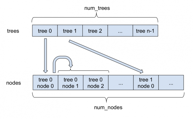
Figure 1 depicts how sparse forests are stored in FIL. All nodes are stored in a single large nodes array. For each tree, the index of its root in the nodes array is stored in the trees array. Each sparse node, in addition to the information stored in a dense node, stores the index of its left child. As each node always has two children, left and right nodes are stored adjacently. Therefore, the index of the right child can always be obtained by adding 1 to the index of the left child. Internally, FIL continues to support dense as well as sparse nodes, with both approaches deriving from a base forest class.
Compared to the internal changes, the changes to the Python API have been kept to a minimum. The new storage_type parameter specifies whether to create a dense or sparse forest. Additionally, a new value,'AUTO', has been made the new default for the inference algorithm parameter; it allows FIL to choose the inference algorithm itself. For sparse forests, it currently uses the'NAIVE'algorithm, which is the only one supported. For dense forests, it uses the'BATCH_TREE_REORG' algorithm.
Benchmarks
To benchmark the sparse trees, we train a random forest using scikit-learn, specifically,sklearn.ensemble.RandomForestClassifier. We then convert the resulting model into a FIL forest and benchmark the performance of inference. The data is generated using sklearn.datasets.make_classification(), and contains 2 million rows split equally between training and validation dataset, and 32 columns. For benchmarking, inference is performed on 1 million rows.
We use two sets of parameters for benchmarking.
- With the depth limit, set to either 10 or 20; in this case, either a dense or sparse FIL forest can fit into GPU memory.
- Without depth limit; in this case, the model trained by SKLearn contains really deep trees. In our benchmark runs, the trees usually have a depth between 30 and 50. Trying to create a dense FIL forest runs out of memory, but a sparse forest can be created smoothly.
In both cases, the size of the forest itself remains relatively small, as the number of leaf nodes in a tree is limited to 2048, and the forest consists of 100 trees. We measure the time of the CPU inference and the GPU inference. The GPU inference was performed on V100, and the CPU inference was performed on a system with 2 sockets, each with 16 cores with 2-way hyperthreading. The benchmark results are presented in Figure 2.
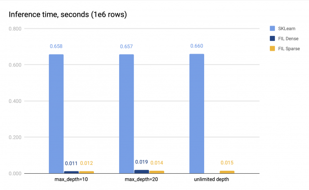
Both sparse and dense FIL predictors (if the latter is available) are about 34–60x faster than the SKLearn CPU predictor. The sparse FIL predictor is slower compared to the dense one for shallow forests, but can be faster for deeper forests; the exact performance difference varies. For instance, in Figure 2 with max_depth=10, the dense predictor is about 1.14x faster than the sparse predictor, but with max_depth=20, it is slower, achieving only 0.75x speed of the sparse predictor. Therefore, the dense FIL predictor should be used for shallow forests.
For deep forests, however, the dense predictor runs out of memory, as its space requirements grow exponentially with the forest depth. The sparse predictor does not have this problem and provides fast inference on the GPU even for very deep trees.
Conclusion
With sparse forest support, FIL applies to a wider range of problems. Whether you’re building gradient-boosted decision trees with XGBoost or random forests with cuML or scikit-learn, FIL should be an easy drop-in option to accelerate your inference. As always, if you encounter any issues, feel free to file issues on GitHub or ask questions in our public Slack channel!