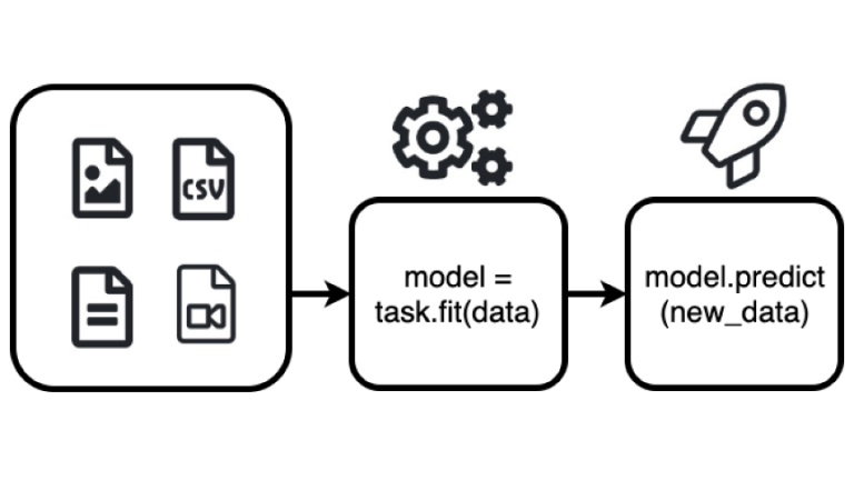
 To achieve state-of-the-art machine learning (ML) solutions, data scientists often build complex ML models. However, these techniques are computationally expensive, and until recently required extensive background knowledge, experience, and human effort. Recently, at GTC21, AWS Senior Data Scientist Nick Erickson gave a session sharing how the combination of AutoGluon, RAPIDS, and NVIDIA GPU computing simplifies … Continued
To achieve state-of-the-art machine learning (ML) solutions, data scientists often build complex ML models. However, these techniques are computationally expensive, and until recently required extensive background knowledge, experience, and human effort.
Recently, at GTC21, AWS Senior Data Scientist Nick Erickson gave a session sharing how the combination of AutoGluon, RAPIDS, and NVIDIA GPU computing simplifies achieving state-of-the-art ML accuracy, while improving performance and lowering costs. This post gives an overview of some key points from Nick’s session:
- What is AutoML and what is different about AutoGluon?
- How does AutoGluon outperform 99% of human data science teams in Kaggle prediction competitions with just three lines of code, without the need for expert knowledge?
- How does the integration of AutoGluon with RAPIDS enable up to 40x faster training and 10x faster inference?
What is AutoGluon?
AutoGluon is an open-source AutoML library that enables easy-to-use and easy-to-extend AutoML with a focus on automated stack ensembling, deep learning, and real-world applications spanning text, image, and tabular data. Intended for both ML beginners and experts, AutoGluon enables you to:
- Quickly prototype deep learning and classical ML solutions for your raw data with a few lines of code.
- Automatically utilize state-of-the-art techniques (where appropriate) without expert knowledge.
- Leverage automatic hyperparameter tuning, model selection/ensembling, architecture search, and data processing.
- Easily improve/tune your bespoke models and data pipelines, or customize AutoGluon for your use case.
This post focuses on AutoGluon-Tabular, an AutoGluon API that requires only a few lines of Python to train highly accurate machine learning models on an unprocessed tabular dataset such as a CSV file. In order to understand how AutoGluon-Tabular does this, we will first explain some concepts.
What is Supervised Machine Learning?
Supervised machine learning takes a set of labelled training instances as input and builds a model that aims to correctly predict the label of each training example based on other information that we know about the example (known as features of the instance). The purpose of this is to build an accurate model that can automatically label future data with unknown labels.

In tabular datasets, columns represent the measurements of a variable (a.k.a. feature), and rows represent individual data points. For example, the table below shows a small dataset with three columns: “has job”, “owns house” and “income”. In this example “income” is the label (sometimes known as the target variable for prediction) and the other columns are features used to try to predict the income.

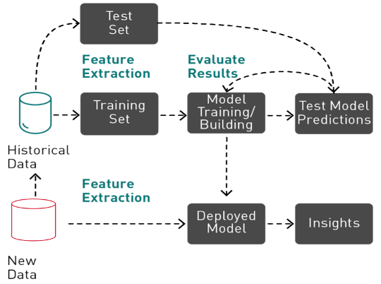
Supervised Machine learning is an iterative, exploratory process that involves Data preparation, feature engineering, validation splitting, missing value handling, training, testing, hyperparameter tuning, ensembling, and evaluating ML models before a model can be used in production to make predictions.
What is AutoML
Historically, achieving state-of-the-art ML performance required extensive background knowledge, experience, and human effort. Depending on the tool and level of automation, AutoML uses different algorithmic techniques to try to find the best features, hyperparameters, algorithms, and or combination of algorithms for an ml pipeline. By automating time-consuming ML pipelines, practitioners and enterprises can apply machine learning to solve business problems faster and more easily.
AutoML in 3 steps with AutoGluon Tabular
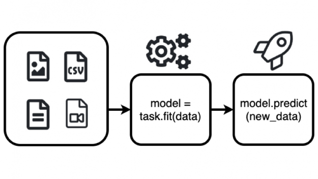
AutoGluon Tabular can be used to automatically build state-of-the-art models that predict a particular column’s value based on the other columns in the same row using two functions: fit (), and predict () as shown below.
from autogluon.tabular import TabularPredictor, TabularDataset
# load dataset
train_data = TabularDataset(DATASET_PATH)
# fit the model
predictor = TabularPredictor(label=LABEL_COLUMN_NAME).fit(train_data)
# make predictions on new data
prediction = predictor.predict(new_data)
The fit() function studies the dataset, performs data preprocessing, fits several models and combines them to produce a high accuracy model. For a more complete example to try out, see the AutoGluon Quick Start tutorial on predicting columns in a table.
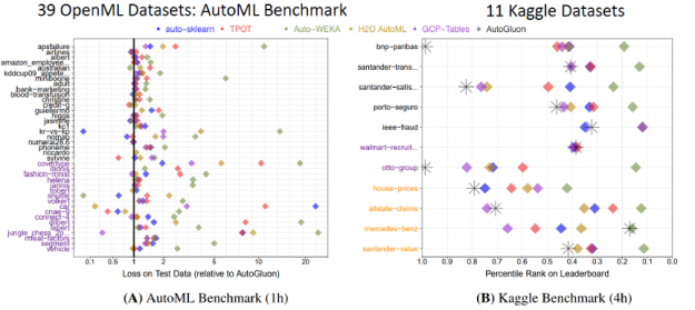
With this simple code, AutoGluon beats other AutoML frameworks and many top data scientists. An extensive evaluation with tests on a suite of 50 classification and regression tasks from Kaggle and the OpenML AutoML Benchmark revealed that AutoGluon is faster, more robust, and more accurate than TPOT, H2O, AutoWEKA, auto-sklearn, and Google AutoML Tables. Also in two popular Kaggle competitions, AutoGluon beat 99% of the participating data scientists after merely 4 hours of training on the raw data.
What is different about AutoGluon?
Most AutoML frameworks focus on the task of Combined Algorithm Selection and Hyperparameter optimization (CASH), offering strategies to find the best model and its hyperparameters from a wide selection of possibilities. However, CASH has some drawbacks:
- It requires many repeated model training and most of the models are thrown away without contributing to the final result.
- The more hyperparameter tuning is done, the higher the risk of overfitting the validation data.
- Hyperparameter tuning is less helpful when ensembling.
In contrast, AutoGluon-Tabular outperforms other frameworks by relying on methods used by expert data scientists to win competitions: ensembling multiple models and stacking them in multiple layers.
How does Ensembling Work?
Ensemble learning methods combine multiple machine learning (ML) algorithms to obtain a better model. To understand this better, let’s go over Random Forests, which is an ensemble of decision trees.
Decision trees create a model that predicts the target label by evaluating a tree of if-then-else and true/false feature questions and estimating the minimum number of questions needed to assess the probability of making a correct decision. Decision trees can be used for classification to predict a category or regression to predict a continuous numeric value. For example, the decision tree below (based on the table above) , tries to predict the label “income” using two decision nodes for the features “has job” and “owns house”.
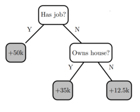
Decision trees have the advantage that they are easy to interpret, but they have problems with overfitting and accuracy. Building an accurate model is somewhere in between underfitting and overfitting —where the model predictions match how the training data behaves and is also generalized enough to make accurate predictions on unseen data.
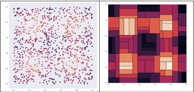
Decision trees seek to find the best split to subset the data, which results in harsh splits. For example, given the dataset below on the left we want to predict the color of a dot where the lighter the dot is the higher the value. A decision tree, shown on the right, would split the data into harsh chunks. Next we will look at how to improve on decision trees with ensembling.
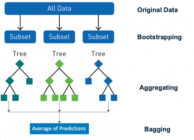
Ensembling is a proven approach to improve the accuracy of models, by combining their predictions and improving generalization. Random forest is a popular ensemble learning method for classification and regression. Random forest uses a technique called bagging (bootstrap aggregating) to build full decision trees in parallel from random bootstrap samples of the data set and features. Predictions are made by aggregating the output from all the trees, which reduces the variance and improves the predictive accuracy. The final prediction is a majority class or mean regression of all the decision tree predictions. Randomness is critical to the success of the forest, bagging makes sure that no decision trees are the same, reducing the problems of overfitting seen with individual trees.
To understand how this gives better predictions, let’s look at an example. Here, are four different decision trees for the data set seen in figure 6, with different prediction colors for a test data point. We can see that each gives approximations of the solution which are not generalized enough to make accurate predictions.
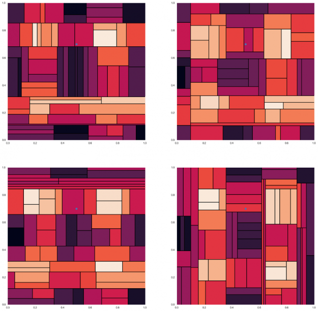
image reference https://gist.github.com/tylerwx51/fc8b316337833c877785222d463a45b0
When these four decision trees are combined and averaged together the harsh boundaries go away and are smoothed as in the random forest example below. Now the prediction color for the test data point is a blend of the colors from the other tree predictions.
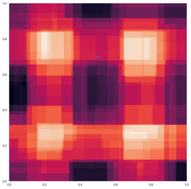
All of the decision trees in a random forest are suboptimal, they are all wrong in random directions. When you average the decision trees, the reasons they are wrong cancel out each other, this is called variance cancellation. The results are of higher quality because they reflect decisions reached by the majority of trees. The averaging limits errors, even though some trees are wrong, others will be right, so the group of trees collectively moves in the correct direction.
When many uncorrelated decision trees are combined, they produce models with high predictive power resilient to over-fitting. These concepts are foundational to popular machine learning algorithms such as Random Forest, XGBoost, Catboost and LightGBM which are employed by AutoGluon.
Multi-layer Stack Ensembling
You can go further than this with ensembling, experienced machine learning practitioners combine outputs of RandomForest, CatBoost, k-nearest neighbors, and others to further improve model accuracy. In the ML competition community it is hard to find a competition won by a single model, every winning solution incorporates ensembles of models.
Stacking is a technique that uses the aggregated predictions of a collection of “base” regression or classification models as the features for training a meta-classifier or regressor “stacker” model.
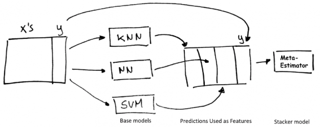
Multi-layer stacking feeds the predictions output by the stacker models as inputs to additional higher layer stacker models. Iterating this process in multiple layers has been a winning strategy in many Kaggle competitions. Multi-layer stacking ensembles are powerful but difficult to use and implement robustly and are not currently utilized by any AutoML framework except Autogluon.
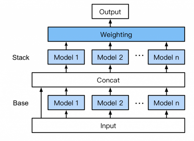
Without the need for expert knowledge, AutoGluon automatically assembles and trains a novel form of multi-layer stack ensembling with k-fold bagging shown in figure 11. Here’s how it works:
- Base: the first layer has multiple base models which are individually trained and bagged using k-fold ensemble bagging (discussed below).
- Concatenating: The base layer model predictions are concatenated along with the input features, to use as input for training the next layer.
- Stacking: Multiple stacker models are trained on the concat layer output. Unlike traditional stacking strategies, AutoGluon reuses the same base layer model types (with the same hyperparameter values) as stackers. Also, the stacker models take as input not only the predictions of the models at the previous layer but also the original data features themselves.
- Weighting: The final stacking layer applies ensemble selection to aggregate the stacker models’ predictions in a weighted manner. Aggregating predictions across a high-capacity stack of models improve resilience against over-fitting
k-fold Ensemble Bagging
AutoGluon improves stacking performance by utilizing all of the available data for both training and validation, through k-fold ensemble bagging of all models at all layers of the stack. k-fold ensemble bagging is similar to k-fold cross validation, which is a method that maximizes the training dataset and is typically used for hyperparameter tuning to determine the best model parameters. With k-fold cross-validation, the data is randomly split into k partitions (folds). Each fold is used one time as the validation dataset, while the rest (Out-Of-Fold – OOF) are used for training. Models are trained using the OOF training sets and evaluated with the validation sets, resulting in k model accuracy measurements. Instead of determining the best model and throwing away the rest, AutoGluon bags all models and obtains OOF predictions from each model on the partition it did not see during training. This creates k-fold predictions of each model which are used as meta-features for the next layer.
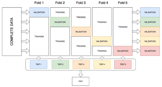
To further improve predictive accuracy and reduce overfitting, AutoGluon-Tabular repeats the k-fold bagging process on n different random partitions of the training data, averaging all OOF predictions over the repeated bags. The number n is chosen by estimating how many rounds can be completed within the specified time constraints when calling the fit() function.
Why AutoGluon Needs GPU Acceleration
Multilayer stack ensembling improves accuracy, however, this means training hundreds of models, a much more compute-intensive task than basic ML use cases, and 10 to 20 times more expensive than weighted ensembling. In the past, the complexity and computational requirements made multilayer stack ensembling difficult to implement for many production use cases and large datasets. With AutoGluon and NVIDIA GPU computing, this is no longer the case.
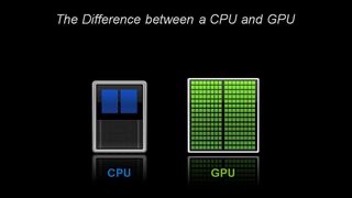
Architecturally, the CPU is composed of just a few cores with lots of cache memory that can handle a few software threads at a time. In contrast, a GPU is composed of hundreds of cores that can handle thousands of threads simultaneously. GPUs have been shown to perform over 20x faster than CPUs in ML workflows and have revolutionized the deep learning field.
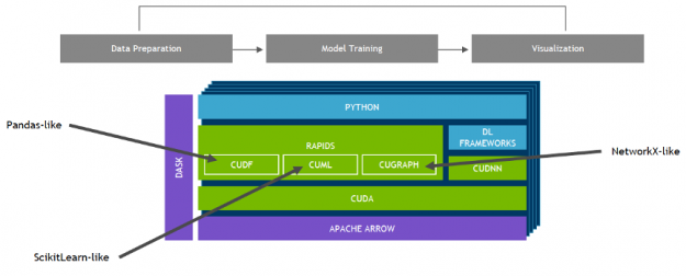
NVIDIA developed RAPIDS—an open-source data analytics and machine learning acceleration platform—for executing end-to-end data science training pipelines completely in GPUs. It relies on NVIDIA® CUDA® primitives for low-level compute optimization, but exposes that GPU parallelism and high memory bandwidth through user-friendly Python interfaces like Pandas and Scikit-Learn APIs.
With RAPIDS’s cuML, popular machine learning algorithms like random forest, XGBoost, and many others are supported for both single-GPU and large data center deployments. For large datasets, these GPU-based implementations can accelerate the training of machine learning models — by up to 45x in the case of random forests, over 100x for support vector machines, and up to 600x for k-nearest neighbors. These speedups can turn overnight jobs into interactive jobs, allow exploration of larger datasets, and enable trying dozens of model variants in the time it would have previously taken to train a single model.
The latest release of AutoGluon leverages the full potential of NVIDIA GPU computing through integration with RAPIDS. With these integrations, AutoGluon is able to train popular ml algorithms on GPUs and increase performance, making highly-performant AutoML accessible to a broader audience.
AutoGluon + RAPIDS Benchmark
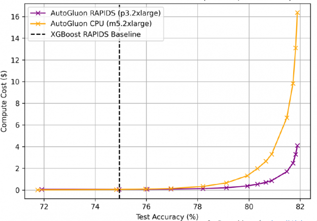
For the 115-million-row airline dataset used in the gradient boosting machines (GBM) benchmarks suite, AutoGluon + RAPIDS accelerated training by 25x compared to AutoGluon on CPUs, with 81.92% accuracy, 7% above the XGBoost baseline. GPUs prefer longer training times as fixed start up costs become less significant.
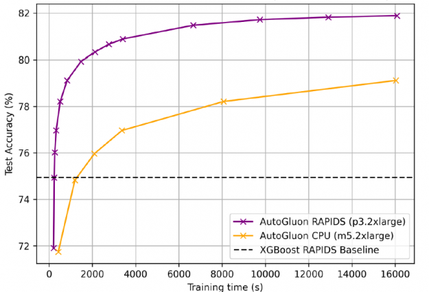
In order to obtain 81.92% accuracy, AutoGluon + RAPIDS on GPUs trained in 4 hours versus 4.5 days for CPUs.
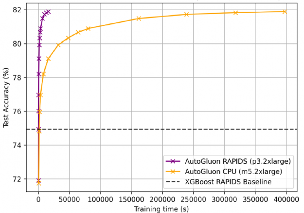
AutoGluon + RAPIDS on GPUs was not only faster, it also cost less, ¼ as much as CPUs to train to the same accuracy (AWS EC2 pricing: p3.2xlarge $0.9180/hr, m5.2xlarge $0.1480/hr).
To Get Started
To get started with AutoGluon and RAPIDS:
- Launch an AWS EC2 instance with p3.2xlarge GPUs
- choose the Deep Learning AMI for CUDA
- Install RAPIDS
- Install AutoGluon-Tabular
- Try out this AutoGluon + RAPIDS Python notebook using data from Otto Group Product Classification Challenge
- The AutoGluon website features numerous tutorials for developers to leverage machine learning for tabular, text, and image data (covering both basic tasks like classification/regression as well as more advanced tasks like object detection).
Conclusion
The AutoGluon AutoML toolkit makes it easy to train and deploy cutting-edge accurate machine learning models for complex business problems. In addition the integration of AutoGluon with RAPIDS leverages the full potential of NVIDIA GPU computing, enabling complex models to train up to 40x faster and predict 10x faster.
For more information, see the following resource
- GTC presentation from Nick Erickson at AWS.
- AutoGluon Website
- AutoGluon Github Repository
- More Progress for Big Impact in the Latest RAPIDS Release
- RAPIDS Accelerates Data Science End-to-End
- Accelerating Random Forests Up to 45x Using cuML
- Gradient Boosting, Decision Trees, and XGBoost with CUDA
- Fast, Accurate, and Simple Models for Tabular Data via Augmented Distillation whitepaper
- AutoGluon-Tabular: Robust and Accurate AutoML for Structured Data whitepaper
- XGBoost on GPUs
- Relentlessly Improving Performance | by Josh Patterson | RAPIDS AI
