Training and Optimizing a 2D Pose Estimation Model with the NVIDIA Transfer Learning Toolkit, Part 1

Human pose estimation is a popular computer vision task of estimating key points on a person’s body such as eyes, arms, and legs. This can help classify a person’s actions, such as standing, sitting, walking, lying down, jumping, and so on. Understanding the context of what a person might be doing in a scene has … Continued

Human pose estimation is a popular computer vision task of estimating key points on a person’s body such as eyes, arms, and legs. This can help classify a person’s actions, such as standing, sitting, walking, lying down, jumping, and so on.

Understanding the context of what a person might be doing in a scene has broad application across a wide range of industries. In a retail setting, this information can be used to understand customer behavior, enhance security, and provide richer analytics. In healthcare, this can be used to monitor patients and alert medical personnel if the patient needs immediate attention. On a factory floor, human pose can be used to identify if proper safety protocols are being followed.

In general, this is a reliable approach in applications that require understanding of human activity and commonly used as one of the key components in more complex tasks such as gesture, tracking, anomaly detection, and so on.

Open-source methods of developing pose estimation exist but are not optimal in terms of inference performance and are time consuming to integrate into production applications. With this post, we show you how to develop and deploy pose estimation models that are easy to use across device profiles, perform extremely well, and are highly accurate.

Pose estimation has been integrated with the NVIDIA Transfer Learning Toolkit (TLT) 3.0 so that you can take advantage of all the TLT features, like model pruning and quantization, to create both an accurate and a high-performance model. After it’s trained, you can deploy this model for inference for real-time performance.

This post series walks you through the steps of training, optimizing, deploying a real-time high performance pose estimation model. In part 1, you learn how to train a 2D pose estimation model using open-source COCO dataset. In part 2, you learn how to optimize the model for inference throughput and then deploy the model using TLT CV inference pipeline. We compare the trained model from TLT with other state-of-the-art models.

Training a 2D Pose Estimation model with TLT

In this section, we cover the following topics on training a 2D pose estimation model with TLT:

• Methodology
• Environment setup
• Data preparation
• Experiment configuration file
• Training
• Evaluation
• Model verification

Methodology

The BodyPoseNet model aims to predict the skeleton for every person in a given input image, which consists of keypoints and the connections between them.

The two commonly used approaches to pose estimation are top-down and bottom-up. A top-down approach typically uses an object detection network to localize the bounding boxes of all humans in a frame, and then uses a pose network to localize the body parts within that bounding box. A bottom-up approach, as the name suggests, builds the skeleton from bottom-up. It first detects all human body parts within a frame and then uses a methodology to group the parts that belong to a specific person.

There are several reasons to adopt a bottom-up approach. One is higher inference performance. With a bottom-up approach, there is no need for a separate person detector, unlike top-down pose estimation methods. The compute does not scale linearly with the number of persons in the scene. This enables you to achieve real-time performance for crowded scenes as well. Moreover, bottom-up also has the advantage of having global context as the entire image is provided as input to the network. It can handle complex poses and crowding better.

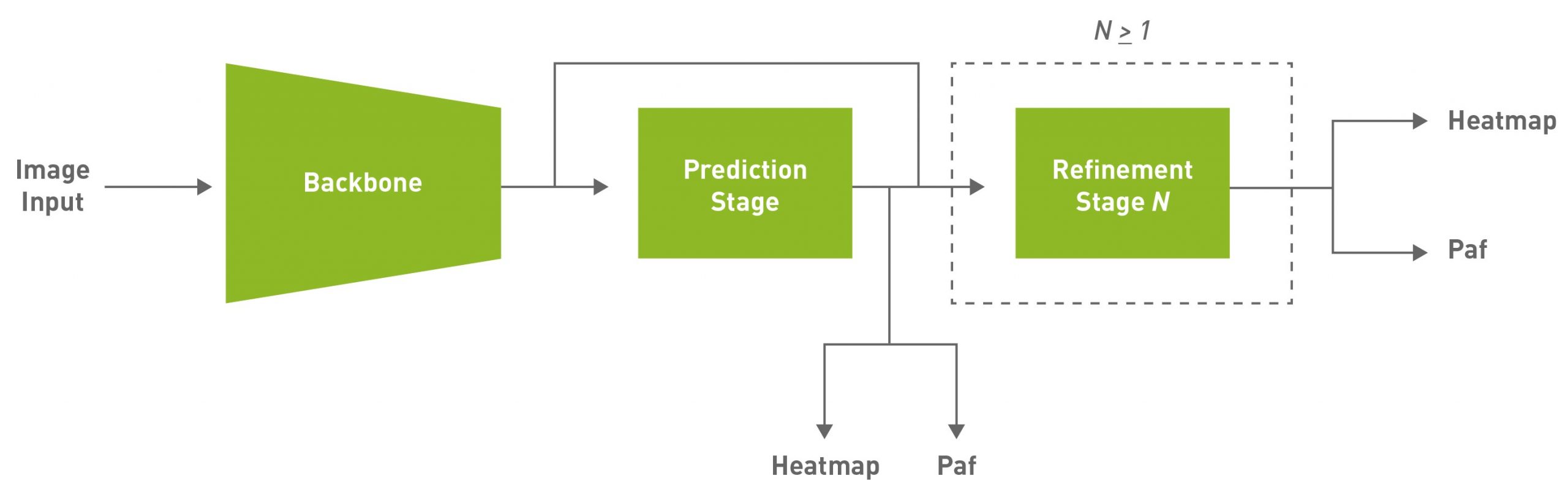
Given some of those reasons, this approach aims to achieve efficient single-shot, bottom-up pose estimation while also delivering competitive accuracy. The default model used in this post is a fully convolutional model and consists of a backbone network, an initial prediction stage which does a pixel-wise prediction of confidence maps (heatmap) and part-affinity fields (PAF) followed by multistage refinement (0 to N stages) on the initial predictions. This solution simplifies and abstracts much of the complexities of the bottom-up approach while allowing for the necessary knobs to be tuned for specific applications.

PAFs are one way to represent association scores in a bottom-up approach. For more information, see Realtime Multi-Person 2D Pose Estimation using Part Affinity Fields. It consists of a set of 2D vector fields that encode the location and orientation of limbs. This, in association with the heatmap, is used to build up the skeleton during post-processing by performing a bipartite matching and associating body part candidates.

Environment setup

NVIDIA TLT toolkit helps abstract away the AI/DL framework complexity and enables you to build production quality models faster, with no coding required. For more information about hardware and software requirements, setting up required dependencies, and installing the TLT launcher, see the TLT Quick Start Guide.

Download the latest samples using the following command:

ngc registry resource download-version "nvidia/tlt_cv_samples:v1.1.0"

You can find the sample notebook located at tlt_cv_samples:v1.1.0/bpnet, which also includes all the steps in detail.

Set up env variables for cleaner command line commands. Update the following variable values:

 export KEY= 
 export NUM_GPUS=1 
 # Local paths
 # The dataset is expected to be present in $LOCAL_PROJECT_DIR/bpnet/data. 
 export LOCAL_PROJECT_DIR=/home//tlt-experiments
 export SAMPLES_DIR=/home//tlt_cv_samples_vv1.1.0
 # Container paths
 export USER_EXPERIMENT_DIR=/workspace/tlt-experiments/bpnet
 export DATA_DIR=/workspace/tlt-experiments/bpnet/data
 export SPECS_DIR=/workspace/examples/bpnet/specs
 export DATA_POSE_SPECS_DIR=/workspace/examples/bpnet/data_pose_config
 export MODEL_POSE_SPECS_DIR=/workspace/examples/bpnet/model_pose_config 

To run the TLT launcher, map the ~/tlt-experiments directory on the local machine to the Docker container using the ~/.tlt_mounts.json file. For more information, see TLT Launcher.

Create the ~/.tlt_mounts.json file and update the following content inside:

 {
     "Mounts": [
         {
             "source": "/home//tlt-experiments",
             "destination": "/workspace/tlt-experiments"
         },
         {
             "source": "/home//tlt_cv_samples_vv1.1.0/bpnet/specs",
             "destination": "/workspace/examples/bpnet/specs"
         },
         {
             "source": "/home//tlt_cv_samples_vv1.1.0/bpnet/data_pose_config",
             "destination": "/workspace/examples/bpnet/data_pose_config"
         },
         {
             "source": "/home//tlt_cv_samples_vv1.1.0/bpnet/model_pose_config",
             "destination": "/workspace/examples/bpnet/model_pose_config"
         }
     ]
 } 

Make sure that the source directory paths to be mounted are valid. This mounts the path /home//tlt-experiments on the host machine to be the path /workspace/tlt-experiments inside the container. It also mounts the downloaded specs on the host machine to be the path /workspace/examples/bpnet/specs, /workspace/examples/bpnet/data_pose_config, and /workspace/examples/bpnet/model_pose_config inside the container.

Make sure that you have installed the required dependencies by running the following command:

 # Install requirements 
 pip3 install -r $SAMPLES_DIR/deps/requirements-pip.txt 

Download the pretrained model

To get started, set up an NGC account and then download the pretrained model. Currently, only the vgg19 backbone is supported.

 # Create the target destination to download the model. 
 mkdir -p $LOCAL_EXPERIMENT_DIR/pretrained_vgg19/
  
 # Download the pretrained model from NGC
 ngc registry model download-version nvidia/tlt_bodyposenet:vgg19 
     --dest $LOCAL_EXPERIMENT_DIR/pretrained_vgg19 

Data preparation

We use the COCO (common objects on context) 2017 dataset in this post as an example. Download the dataset and extract as per the instructions:

• train_data
• val_data
• annotations

Unzip the images directories into the $LOCAL_DATA_DIR directory and the annotations into $LOCAL_DATA_DIR/annotations.

To prepare the data for training, you must generate segmentation masks to be used for masking the loss of unlabeled persons and tfrecords to feed to the training pipeline. The mask folder is based on the path provided in the coco_spec.json file. mask_root_dir_path directory is a relative path to root_directory_path, as are mask_root_dir_path and annotation_root_dir_path.

 # Generate TFRecords for training dataset
 tlt bpnet dataset_convert 
         -m 'train' 
         -o $DATA_DIR/train 
         --generate_masks 
         --dataset_spec $DATA_POSE_SPECS_DIR/coco_spec.json
  
 # Generate TFRecords for validation dataset 
 tlt bpnet dataset_convert  
         -m 'test' 
         -o $DATA_DIR/val 
         --generate_masks  
         --dataset_spec $DATA_POSE_SPECS_DIR/coco_spec.json 

To use this example with a custom dataset:

• Prepare the data and annotations in a format similar to the COCO dataset.
• Create a dataset spec under data_pose_config, similar to coco_spec.json, that includes the dataset paths, pose configuration, occlusion labeling convention, and so on.
• Convert your annotations to the COCO annotations format.

For more information, see the following docs:

• COCO data format
• Explanation of the data format
• Creating a Configuration File for the Dataset Converter

Train experiment configuration file

The next step is to configure the spec file for training. The experiment spec file is essential, as it compiles all the necessary hyperparameters for achieving a good model. The specification file for BodyPoseNet training configures these components of the training pipe:

• Trainer
• Dataloader
• Augmentation
• Label Processor
• Model
• Optimizer

You can find the default specification file at $SPECS_DIR/bpnet_train_m1_coco.yaml. We expand on each component of the specification file but we don’t cover all the parameters here. For more information, see Create a Train Experiment Configuration File.

Trainer (Top-level config)

The top-level experiment configs include basic parameters for an experiment; for example, number of epochs, pretrained weights, whether to load the pretrained graph, and so on. An encrypted checkpoint is saved per the checkpoint_n_epoch value. Here’s a code example of some of the top-level configs.

checkpoint_dir: /workspace/tlt-experiments/bpnet/models/exp_m1_unpruned
 checkpoint_n_epoch: 5
 num_epoch: 100
 pretrained_weights: /workspace/tlt-experiments/bpnet/pretrained_vgg19/tlt_bodyposenet_vvgg19/vgg_19.hdf5
 load_graph: False
 use_stagewise_lr_multipliers: True
 ... 

All the paths (checkpoint_dir and pretrained_weights) are internal to the Docker container. To verify correctness, check ~/.tlt_mounts.json. For more information about these parameters, see the Body Pose Trainer section.

Dataloader

This section helps you with defining datapaths, image configuration, the target pose configuration, normalization parameters, and so on. The augmentation_config section provides some on-the-fly augmentation options. It supports basic spatial augmentations, such as flip, zoom, rotate, and translate, which can be configured before training experiments. The label_processor_config section provides the required parameters to configure the ground truth feature map generation.

dataloader:
   batch_size: 10
   pose_config:
     target_shape: [32, 32]
     pose_config_path: /workspace/examples/bpnet/model_pose_config/bpnet_18joints.json
   image_config:
     image_dims:
       height: 256
       width: 256
       channels: 3
     image_encoding: jpg
   dataset_config:
     root_data_path: /workspace/tlt-experiments/bpnet/data/
     train_records_folder_path: /workspace/tlt-experiments/bpnet/data
     train_records_path: [train-fold-000-of-001]
     dataset_specs:
       coco: /workspace/examples/bpnet/data_pose_config/coco_spec.json
   normalization_params: 
     ...
   augmentation_config:
     spatial_augmentation_mode: person_centric
     spatial_aug_params:
       flip_lr_prob: 0.5
       flip_tb_prob: 0.0
       ...
   label_processor_config:
     paf_gaussian_sigma: 0.03
     heatmap_gaussian_sigma: 7.0
     paf_ortho_dist_thresh: 1.0 

• The target_shape value depends on the image_dims and model stride values (target_shape = input_shape / model stride). The current model has a stride of 8.
• Make sure to use the same root_data_path value as root_directory_path in dataset_spec. The mask and image data directories in dataset_spec are relative to root_data_path.
• All paths, including pose_config_path, dataset_config, and dataset_specs, are internal to Docker.
• Several spatial_augmentation_modes are supported:
  • person_centric: Augmentations are centered around a person of interest in the ground truth.
  • standard: Augmentations are standard (that is, centered around the center of the image) and the aspect ratio of the image is retained.
  • standard_with_fixed_aspect_ratio: Same as standard, but the aspect ratio is fixed to the network input aspect ratio.

For more information about each parameter, see the Dataloader section.

Model

The BodyPoseNet model can be configured using the model option in the spec file. The following is a sample model config to instantiate a custom VGG19-backbone-based model.

model:
  backbone_attributes:
    architecture: vgg
  stages: 3
  heat_channels: 19
  paf_channels: 38
  use_self_attention: False
  data_format: channels_last
  use_bias: True
  regularization_type: l1
  kernel_regularization_factor: 5.0e-4
  bias_regularization_factor: 0.0
  ... 

The number of total stages for pose estimation (stages of refinement + 1) in the network is captured by the stages param which takes any value >= 2. We recommend using the L1 regularizer when training a network before pruning, as L1 regularization makes it easier to prune the network weights. For more information about each parameter in the model, see the Model section.

Optimizer

This section describes how to configure the optimizer and learning-rate schedule:

optimizer:
   __class_name__: WeightedMomentumOptimizer
   learning_rate_schedule:
     __class_name__: SoftstartAnnealingLearningRateSchedule
     soft_start: 0.05
     annealing: 0.5
     base_learning_rate: 2.e-5
     min_learning_rate: 8.e-08
   momentum: 0.9
   use_nesterov: False 

The default base_learning_rate is set for a single-GPU training. To use multi-GPU training, you may have to modify the learning_rate value to get similar accuracy. In most cases, scaling up the learning rate by a factor of $NUM_GPUS would be a good start. For instance, if you are using two GPUs, use 2 * base_learning_rate used in one GPU setting, and if you are using four GPUs, use 4 * base_learning_rate. For more information about each parameter in the model, see the Optimizer section.

Training

After following the steps to generate TFRecords and masks and setting up a train specification file, you are now ready to start training the body pose estimation network. Use the following command to launch training:

tlt bpnet train -e $SPECS_DIR/bpnet_train_m1_coco.yaml 
                 -r $USER_EXPERIMENT_DIR/models/exp_m1_unpruned 
                 -k $KEY 
                 --gpus $NUM_GPUS 

Training with more GPUs enables networks to ingest more data faster, saving you precious time during the development process. TLT supports multi-GPU training so that you can train the model with several GPUs in parallel. We recommend using four GPUs or more for training the model as one GPU might take several days to complete. The training time roughly decreases by a factor of $NUM_GPUS. Make sure that you update the learning rates accordingly, based on the linear scaling method described in the Optimizer section.

BodyPoseNet supports restarting from checkpoint. In case the training job is killed prematurely, you may resume training from the last saved checkpoint by simply rerunning the same command. Make sure that you use the same number of GPUs when restarting the training.

Evaluation

Start with configuring the inference and evaluation specification file. The following code example is a sample specification:

model_path: /workspace/tlt-experiments/bpnet/models/exp_m1_unpruned/bpnet_model.tlt
 train_spec: /workspace/examples/bpnet/specs/bpnet_train_m1_coco.yaml
 input_shape: [368, 368]
 # choose from: {pad_image_input, adjust_network_input, None}
 keep_aspect_ratio_mode: adjust_network_input
 output_stage_to_use: null
 output_upsampling_factor: [8, 8]
 heatmap_threshold: 0.1
 paf_threshold: 0.05
 multi_scale_inference: False
 scales: [0.5, 1.0, 1.5, 2.0] 

The value of input_shape here can be different from the input_dims value used for training. The multi_scale_inference parameter enables multiscale refinement over the provided scales. Because you are using a model of stride 8, output_upsampling_factor is set to 8.

To keep the evaluation consistent with bottom-up human pose estimation research, there are two modes and specification files to evaluate the model:

• $SPECS_DIR/infer_spec.yaml: Single-scale, nonstrict input. This configuration does a single-scale inference on the input image. The aspect ratio of the input image is retained by fixing one of the sides of the network input (height or width), and adjusting the other side to match the aspect ratio of the input image.
• $SPECS_DIR/infer_spec_refine.yaml: Multiscale, nonstrict input. This configuration does a multiscale inference on the input image. The scales are configurable.

There is another mode used primarily to verify against the final exported TRT models. You use this in later sections.

• $SPECS_DIR/infer_spec_strict.yaml: Single-scale, strict input. This configuration does a single-scale inference on the input image. Aspect ratio of the input image is retained by padding the image on the sides as needed to fit the network input size as the TRT model input dims are fixed.

The --model_filename argument overrides the model_path variable in the inference specification file.

To evaluate the model, use the following command:

# Single-scale evaluation
 tlt bpnet evaluate --inference_spec $SPECS_DIR/infer_spec.yaml 
                    --model_filename $USER_EXPERIMENT_DIR/models/exp_m1_unpruned/$MODEL_CHECKPOINT 
                    --dataset_spec $DATA_POSE_SPECS_DIR/coco_spec.json 
                    --results_dir $USER_EXPERIMENT_DIR/results/exp_m1_unpruned/eval_default 
                    -k $KEY 

Model verification

Now that you’ve trained the model, run inference and verify the predictions. To verify the model visually with TLT, use the tlt bpnet inference command. The tool supports running inference on the .tlt model, as well as the TensorRT .engine model. It generates annotated images with skeleton rendered on them and serialized frame-by-frame keypoint labels and metadata in detections.json. For example, to run inference with a trained .tlt model, run the following command:

tlt bpnet inference --inference_spec $SPECS_DIR/infer_spec.yaml 
                     --model_filename $USER_EXPERIMENT_DIR/models/exp_m1_unpruned/$MODEL_CHECKPOINT 
                     --input_type dir 
                     --input $USER_EXPERIMENT_DIR/data/sample_images 
                     --results_dir $USER_EXPERIMENT_DIR/results/exp_m1_unpruned/infer_default 
                     --dump_visualizations 
                     -k $KEY 

Figure 1 shows an example of the original image and Figure 2 shows the output image with pose results rendered. As you can see, the model is robust to an image that is different from the COCO training data.

Conclusion

In this post, you learned about training body pose models using the BodyPoseNet app in TLT. The post showed taking an open-source COCO dataset with a pretrained backbone from NGC to train a model with TLT. To optimize the trained model for inference and deployment, see Training and Optimizing the 2D Pose Estimation Model, Part 2.

For more information, see the following resources:

• Body Pose Estimation Training
• TLT Getting Started Guide
• Transfer Learning Toolkit
• TLT CV Inference Pipeline