Month: June 2021

As explained in the Batch Normalization paper, training neural networks becomes way easier if its input is Gaussian. This is clear. And if your model inputs are not Gaussian, RAPIDS will just transform it to Gaussian in the blink of an eye. Gauss rank transformation is a novel standardization technique to transform input data for … Continued

As explained in the Batch Normalization paper, training neural networks becomes way easier if its input is Gaussian. This is clear. And if your model inputs are not Gaussian, RAPIDS will just transform it to Gaussian in the blink of an eye.

Gauss rank transformation is a novel standardization technique to transform input data for training deep neural networks. Recently, we used this technique in the Predicting Molecular Properties competition and it easily boosted the accuracy of the message passing neural network model by a significant margin. This blog post will show how simple it is to implement a GPU-accelerated Gauss rank transformation with drop-in replacements of Pandas and NumPy using RAPIDS cuDF and Chainer CuPy to deliver 100x speedup.

Introduction

Input normalization is critical for training neural nets. The idea of Gauss rank transformation was first introduced by Michael Jahrer in his winning solution of Porto Seguro’s Safe Driver Prediction challenge. He trained denoising auto-encoders and experimented with several input normalization methods. In the end, he drew this conclusion:

The best thing I found during the past and works straight out of the box is GaussRank. This works usually much better than standard mean/std scaler or min/max (normalization).

How it works

There are three steps to transform a vector of continuous values under arbitrary distribution to Gaussian distribution based on ranks, as shown in the figure 1.

The CuPy implementation is straightforward and remarkably resembles NumPy operations. In fact, it is as simple as changing the imported functions to move the whole process from CPU to GPU without any other code changes.

View this code snippet on GitHub.

Inverse Transformation is used to restore the original values from the Gaussian transformations. This is another great example to show the interoperability of cuDF and CuPy. Just like you can do with NumPy and Pandas, you can weave cuDF and CuPy together in the same workflow while keeping the data entirely on the GPU.

View this code snippet on GitHub.

A real-world example

For this example, we will use the CHAMPS molecular properties prediction dataset. The task is to predict scalar coupling constants (the ground truth) between atom pairs in molecules for eight different chemical bond types. What’s challenging is that the distribution of the ground truth differs significantly for each bond type, with varied mean and variance. This makes it difficult for the neural network to converge.

Hence, we applied the Gauss rank transformation to the ground truths of training data to create one unified clean Gaussian distribution for all bond types.

In this regression task, ground truths of training data are transformed using GaussRank.

For inference, we applied the inverse Gauss rank transformation to the predictions of the test data so that they match the original different distributions for each bond type. Since the true distribution of targets of the test data is unknown, the inverse transformation of the predictions of the test data is calculated based on the distribution of target variables in training data. It should be noted that such an inverse transformation is only needed for target variables.

By applying this single trick, the Log of the Mean Absolute Error (LMAE) of our message passing neural network is improved by 18%!

Keep in mind that GaussRank does have some limitations:

• It works only for continuous variables, and
• if the input is already close to Gaussian, or very asymmetrical, performance might not be improved or even become worse.

The interplay between gauss rank transformation and different kinds of neural networks is an active research topic.

Speedup

We measure the total time of transformation and the inverse transformation. For the proceeding CHAMPS dataset, the cuDF+CuPy implementation on a single NVIDIA V100 GPU achieves 25x speedup over the Pandas+NumPy implementation on an Intel Xeon CPU. We generate synthetic random data for a more comprehensive comparison. For 10M data points and more, our RAPIDS implementation is more than 100x faster.

Conclusion

RAPIDS has come a long way to deliver stunning performance with little or no code changes. This blog post showcases how easy it is to use RAPIDS cuDF and CuPy as drop-in replacements to Pandas and NumPy to realize the performance improvements on GPUs. As shown in the full notebook, by adding just two lines of code, the Gauss rank transformation detects the input tensor is on GPU and automatically switches to cuDF+CuPy from Pandas+NumPy. It can’t be much easier than that.

submitted by /u/flowreaction
[visit reddit] [comments]

submitted by /u/LivingPornFree
[visit reddit] [comments]

submitted by /u/grid_world
[visit reddit] [comments]

Human pose estimation is a popular computer vision task of estimating key points on a person’s body such as eyes, arms, and legs. This can help classify a person’s actions, such as standing, sitting, walking, lying down, jumping, and so on. Understanding the context of what a person might be doing in a scene has … Continued

Human pose estimation is a popular computer vision task of estimating key points on a person’s body such as eyes, arms, and legs. This can help classify a person’s actions, such as standing, sitting, walking, lying down, jumping, and so on.

Understanding the context of what a person might be doing in a scene has broad application across a wide range of industries. In a retail setting, this information can be used to understand customer behavior, enhance security, and provide richer analytics. In healthcare, this can be used to monitor patients and alert medical personnel if the patient needs immediate attention. On a factory floor, human pose can be used to identify if proper safety protocols are being followed.

In general, this is a reliable approach in applications that require understanding of human activity and commonly used as one of the key components in more complex tasks such as gesture, tracking, anomaly detection, and so on.

Open-source methods of developing pose estimation exist but are not optimal in terms of inference performance and are time consuming to integrate into production applications. With this post, we show you how to develop and deploy pose estimation models that are easy to use across device profiles, perform extremely well, and are highly accurate.

Pose estimation has been integrated with the NVIDIA Transfer Learning Toolkit (TLT) 3.0 so that you can take advantage of all the TLT features, like model pruning and quantization, to create both an accurate and a high-performance model. After it’s trained, you can deploy this model for inference for real-time performance.

This post series walks you through the steps of training, optimizing, deploying a real-time high performance pose estimation model. In part 1, you learn how to train a 2D pose estimation model using open-source COCO dataset. In part 2, you learn how to optimize the model for inference throughput and then deploy the model using TLT CV inference pipeline. We compare the trained model from TLT with other state-of-the-art models.

Training a 2D Pose Estimation model with TLT

In this section, we cover the following topics on training a 2D pose estimation model with TLT:

• Methodology
• Environment setup
• Data preparation
• Experiment configuration file
• Training
• Evaluation
• Model verification

Methodology

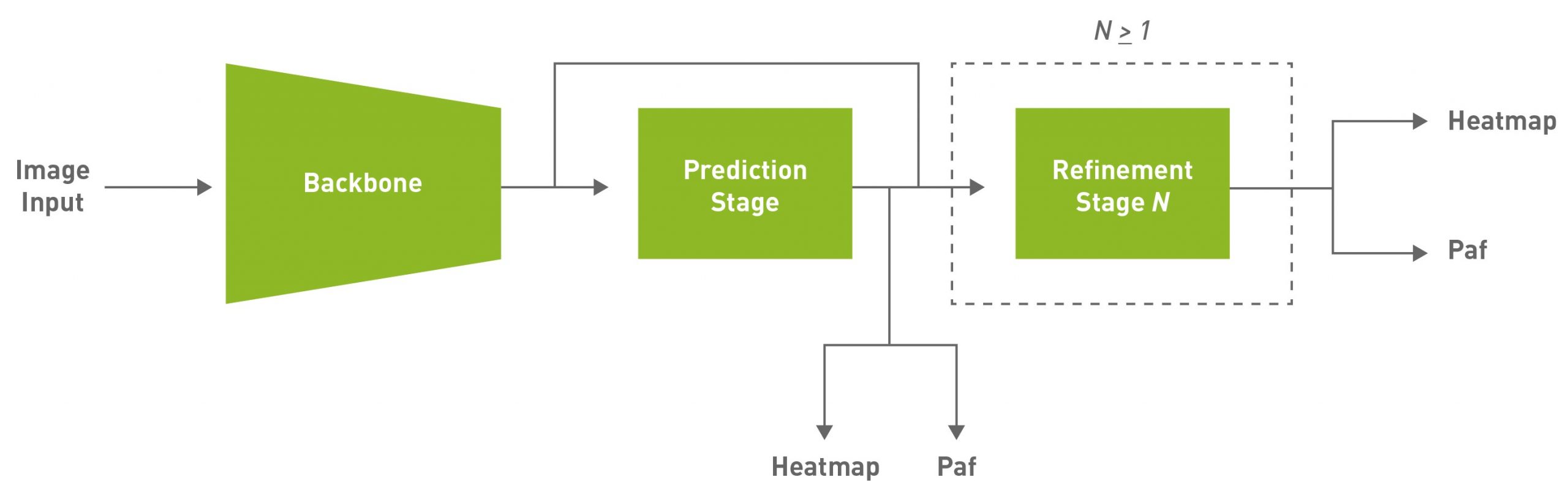
The BodyPoseNet model aims to predict the skeleton for every person in a given input image, which consists of keypoints and the connections between them.

The two commonly used approaches to pose estimation are top-down and bottom-up. A top-down approach typically uses an object detection network to localize the bounding boxes of all humans in a frame, and then uses a pose network to localize the body parts within that bounding box. A bottom-up approach, as the name suggests, builds the skeleton from bottom-up. It first detects all human body parts within a frame and then uses a methodology to group the parts that belong to a specific person.

There are several reasons to adopt a bottom-up approach. One is higher inference performance. With a bottom-up approach, there is no need for a separate person detector, unlike top-down pose estimation methods. The compute does not scale linearly with the number of persons in the scene. This enables you to achieve real-time performance for crowded scenes as well. Moreover, bottom-up also has the advantage of having global context as the entire image is provided as input to the network. It can handle complex poses and crowding better.

Given some of those reasons, this approach aims to achieve efficient single-shot, bottom-up pose estimation while also delivering competitive accuracy. The default model used in this post is a fully convolutional model and consists of a backbone network, an initial prediction stage which does a pixel-wise prediction of confidence maps (heatmap) and part-affinity fields (PAF) followed by multistage refinement (0 to N stages) on the initial predictions. This solution simplifies and abstracts much of the complexities of the bottom-up approach while allowing for the necessary knobs to be tuned for specific applications.

PAFs are one way to represent association scores in a bottom-up approach. For more information, see Realtime Multi-Person 2D Pose Estimation using Part Affinity Fields. It consists of a set of 2D vector fields that encode the location and orientation of limbs. This, in association with the heatmap, is used to build up the skeleton during post-processing by performing a bipartite matching and associating body part candidates.

Environment setup

NVIDIA TLT toolkit helps abstract away the AI/DL framework complexity and enables you to build production quality models faster, with no coding required. For more information about hardware and software requirements, setting up required dependencies, and installing the TLT launcher, see the TLT Quick Start Guide.

Download the latest samples using the following command:

ngc registry resource download-version "nvidia/tlt_cv_samples:v1.1.0"

You can find the sample notebook located at tlt_cv_samples:v1.1.0/bpnet, which also includes all the steps in detail.

Set up env variables for cleaner command line commands. Update the following variable values:

 export KEY= 
 export NUM_GPUS=1 
 # Local paths
 # The dataset is expected to be present in $LOCAL_PROJECT_DIR/bpnet/data. 
 export LOCAL_PROJECT_DIR=/home//tlt-experiments
 export SAMPLES_DIR=/home//tlt_cv_samples_vv1.1.0
 # Container paths
 export USER_EXPERIMENT_DIR=/workspace/tlt-experiments/bpnet
 export DATA_DIR=/workspace/tlt-experiments/bpnet/data
 export SPECS_DIR=/workspace/examples/bpnet/specs
 export DATA_POSE_SPECS_DIR=/workspace/examples/bpnet/data_pose_config
 export MODEL_POSE_SPECS_DIR=/workspace/examples/bpnet/model_pose_config 

To run the TLT launcher, map the ~/tlt-experiments directory on the local machine to the Docker container using the ~/.tlt_mounts.json file. For more information, see TLT Launcher.

Create the ~/.tlt_mounts.json file and update the following content inside:

 {
     "Mounts": [
         {
             "source": "/home//tlt-experiments",
             "destination": "/workspace/tlt-experiments"
         },
         {
             "source": "/home//tlt_cv_samples_vv1.1.0/bpnet/specs",
             "destination": "/workspace/examples/bpnet/specs"
         },
         {
             "source": "/home//tlt_cv_samples_vv1.1.0/bpnet/data_pose_config",
             "destination": "/workspace/examples/bpnet/data_pose_config"
         },
         {
             "source": "/home//tlt_cv_samples_vv1.1.0/bpnet/model_pose_config",
             "destination": "/workspace/examples/bpnet/model_pose_config"
         }
     ]
 } 

Make sure that the source directory paths to be mounted are valid. This mounts the path /home//tlt-experiments on the host machine to be the path /workspace/tlt-experiments inside the container. It also mounts the downloaded specs on the host machine to be the path /workspace/examples/bpnet/specs, /workspace/examples/bpnet/data_pose_config, and /workspace/examples/bpnet/model_pose_config inside the container.

Make sure that you have installed the required dependencies by running the following command:

 # Install requirements 
 pip3 install -r $SAMPLES_DIR/deps/requirements-pip.txt 

Download the pretrained model

To get started, set up an NGC account and then download the pretrained model. Currently, only the vgg19 backbone is supported.

 # Create the target destination to download the model. 
 mkdir -p $LOCAL_EXPERIMENT_DIR/pretrained_vgg19/
  
 # Download the pretrained model from NGC
 ngc registry model download-version nvidia/tlt_bodyposenet:vgg19 
     --dest $LOCAL_EXPERIMENT_DIR/pretrained_vgg19 

Data preparation

We use the COCO (common objects on context) 2017 dataset in this post as an example. Download the dataset and extract as per the instructions:

• train_data
• val_data
• annotations

Unzip the images directories into the $LOCAL_DATA_DIR directory and the annotations into $LOCAL_DATA_DIR/annotations.

To prepare the data for training, you must generate segmentation masks to be used for masking the loss of unlabeled persons and tfrecords to feed to the training pipeline. The mask folder is based on the path provided in the coco_spec.json file. mask_root_dir_path directory is a relative path to root_directory_path, as are mask_root_dir_path and annotation_root_dir_path.

 # Generate TFRecords for training dataset
 tlt bpnet dataset_convert 
         -m 'train' 
         -o $DATA_DIR/train 
         --generate_masks 
         --dataset_spec $DATA_POSE_SPECS_DIR/coco_spec.json
  
 # Generate TFRecords for validation dataset 
 tlt bpnet dataset_convert  
         -m 'test' 
         -o $DATA_DIR/val 
         --generate_masks  
         --dataset_spec $DATA_POSE_SPECS_DIR/coco_spec.json 

To use this example with a custom dataset:

• Prepare the data and annotations in a format similar to the COCO dataset.
• Create a dataset spec under data_pose_config, similar to coco_spec.json, that includes the dataset paths, pose configuration, occlusion labeling convention, and so on.
• Convert your annotations to the COCO annotations format.

For more information, see the following docs:

• COCO data format
• Explanation of the data format
• Creating a Configuration File for the Dataset Converter

Train experiment configuration file

The next step is to configure the spec file for training. The experiment spec file is essential, as it compiles all the necessary hyperparameters for achieving a good model. The specification file for BodyPoseNet training configures these components of the training pipe:

• Trainer
• Dataloader
• Augmentation
• Label Processor
• Model
• Optimizer

You can find the default specification file at $SPECS_DIR/bpnet_train_m1_coco.yaml. We expand on each component of the specification file but we don’t cover all the parameters here. For more information, see Create a Train Experiment Configuration File.

Trainer (Top-level config)

The top-level experiment configs include basic parameters for an experiment; for example, number of epochs, pretrained weights, whether to load the pretrained graph, and so on. An encrypted checkpoint is saved per the checkpoint_n_epoch value. Here’s a code example of some of the top-level configs.

checkpoint_dir: /workspace/tlt-experiments/bpnet/models/exp_m1_unpruned
 checkpoint_n_epoch: 5
 num_epoch: 100
 pretrained_weights: /workspace/tlt-experiments/bpnet/pretrained_vgg19/tlt_bodyposenet_vvgg19/vgg_19.hdf5
 load_graph: False
 use_stagewise_lr_multipliers: True
 ... 

All the paths (checkpoint_dir and pretrained_weights) are internal to the Docker container. To verify correctness, check ~/.tlt_mounts.json. For more information about these parameters, see the Body Pose Trainer section.

Dataloader

This section helps you with defining datapaths, image configuration, the target pose configuration, normalization parameters, and so on. The augmentation_config section provides some on-the-fly augmentation options. It supports basic spatial augmentations, such as flip, zoom, rotate, and translate, which can be configured before training experiments. The label_processor_config section provides the required parameters to configure the ground truth feature map generation.

dataloader:
   batch_size: 10
   pose_config:
     target_shape: [32, 32]
     pose_config_path: /workspace/examples/bpnet/model_pose_config/bpnet_18joints.json
   image_config:
     image_dims:
       height: 256
       width: 256
       channels: 3
     image_encoding: jpg
   dataset_config:
     root_data_path: /workspace/tlt-experiments/bpnet/data/
     train_records_folder_path: /workspace/tlt-experiments/bpnet/data
     train_records_path: [train-fold-000-of-001]
     dataset_specs:
       coco: /workspace/examples/bpnet/data_pose_config/coco_spec.json
   normalization_params: 
     ...
   augmentation_config:
     spatial_augmentation_mode: person_centric
     spatial_aug_params:
       flip_lr_prob: 0.5
       flip_tb_prob: 0.0
       ...
   label_processor_config:
     paf_gaussian_sigma: 0.03
     heatmap_gaussian_sigma: 7.0
     paf_ortho_dist_thresh: 1.0 

• The target_shape value depends on the image_dims and model stride values (target_shape = input_shape / model stride). The current model has a stride of 8.
• Make sure to use the same root_data_path value as root_directory_path in dataset_spec. The mask and image data directories in dataset_spec are relative to root_data_path.
• All paths, including pose_config_path, dataset_config, and dataset_specs, are internal to Docker.
• Several spatial_augmentation_modes are supported:
  • person_centric: Augmentations are centered around a person of interest in the ground truth.
  • standard: Augmentations are standard (that is, centered around the center of the image) and the aspect ratio of the image is retained.
  • standard_with_fixed_aspect_ratio: Same as standard, but the aspect ratio is fixed to the network input aspect ratio.

For more information about each parameter, see the Dataloader section.

Model

The BodyPoseNet model can be configured using the model option in the spec file. The following is a sample model config to instantiate a custom VGG19-backbone-based model.

model:
  backbone_attributes:
    architecture: vgg
  stages: 3
  heat_channels: 19
  paf_channels: 38
  use_self_attention: False
  data_format: channels_last
  use_bias: True
  regularization_type: l1
  kernel_regularization_factor: 5.0e-4
  bias_regularization_factor: 0.0
  ... 

The number of total stages for pose estimation (stages of refinement + 1) in the network is captured by the stages param which takes any value >= 2. We recommend using the L1 regularizer when training a network before pruning, as L1 regularization makes it easier to prune the network weights. For more information about each parameter in the model, see the Model section.

Optimizer

This section describes how to configure the optimizer and learning-rate schedule:

optimizer:
   __class_name__: WeightedMomentumOptimizer
   learning_rate_schedule:
     __class_name__: SoftstartAnnealingLearningRateSchedule
     soft_start: 0.05
     annealing: 0.5
     base_learning_rate: 2.e-5
     min_learning_rate: 8.e-08
   momentum: 0.9
   use_nesterov: False 

The default base_learning_rate is set for a single-GPU training. To use multi-GPU training, you may have to modify the learning_rate value to get similar accuracy. In most cases, scaling up the learning rate by a factor of $NUM_GPUS would be a good start. For instance, if you are using two GPUs, use 2 * base_learning_rate used in one GPU setting, and if you are using four GPUs, use 4 * base_learning_rate. For more information about each parameter in the model, see the Optimizer section.

Training

After following the steps to generate TFRecords and masks and setting up a train specification file, you are now ready to start training the body pose estimation network. Use the following command to launch training:

tlt bpnet train -e $SPECS_DIR/bpnet_train_m1_coco.yaml 
                 -r $USER_EXPERIMENT_DIR/models/exp_m1_unpruned 
                 -k $KEY 
                 --gpus $NUM_GPUS 

Training with more GPUs enables networks to ingest more data faster, saving you precious time during the development process. TLT supports multi-GPU training so that you can train the model with several GPUs in parallel. We recommend using four GPUs or more for training the model as one GPU might take several days to complete. The training time roughly decreases by a factor of $NUM_GPUS. Make sure that you update the learning rates accordingly, based on the linear scaling method described in the Optimizer section.

BodyPoseNet supports restarting from checkpoint. In case the training job is killed prematurely, you may resume training from the last saved checkpoint by simply rerunning the same command. Make sure that you use the same number of GPUs when restarting the training.

Evaluation

Start with configuring the inference and evaluation specification file. The following code example is a sample specification:

model_path: /workspace/tlt-experiments/bpnet/models/exp_m1_unpruned/bpnet_model.tlt
 train_spec: /workspace/examples/bpnet/specs/bpnet_train_m1_coco.yaml
 input_shape: [368, 368]
 # choose from: {pad_image_input, adjust_network_input, None}
 keep_aspect_ratio_mode: adjust_network_input
 output_stage_to_use: null
 output_upsampling_factor: [8, 8]
 heatmap_threshold: 0.1
 paf_threshold: 0.05
 multi_scale_inference: False
 scales: [0.5, 1.0, 1.5, 2.0] 

The value of input_shape here can be different from the input_dims value used for training. The multi_scale_inference parameter enables multiscale refinement over the provided scales. Because you are using a model of stride 8, output_upsampling_factor is set to 8.

To keep the evaluation consistent with bottom-up human pose estimation research, there are two modes and specification files to evaluate the model:

• $SPECS_DIR/infer_spec.yaml: Single-scale, nonstrict input. This configuration does a single-scale inference on the input image. The aspect ratio of the input image is retained by fixing one of the sides of the network input (height or width), and adjusting the other side to match the aspect ratio of the input image.
• $SPECS_DIR/infer_spec_refine.yaml: Multiscale, nonstrict input. This configuration does a multiscale inference on the input image. The scales are configurable.

There is another mode used primarily to verify against the final exported TRT models. You use this in later sections.

• $SPECS_DIR/infer_spec_strict.yaml: Single-scale, strict input. This configuration does a single-scale inference on the input image. Aspect ratio of the input image is retained by padding the image on the sides as needed to fit the network input size as the TRT model input dims are fixed.

The --model_filename argument overrides the model_path variable in the inference specification file.

To evaluate the model, use the following command:

# Single-scale evaluation
 tlt bpnet evaluate --inference_spec $SPECS_DIR/infer_spec.yaml 
                    --model_filename $USER_EXPERIMENT_DIR/models/exp_m1_unpruned/$MODEL_CHECKPOINT 
                    --dataset_spec $DATA_POSE_SPECS_DIR/coco_spec.json 
                    --results_dir $USER_EXPERIMENT_DIR/results/exp_m1_unpruned/eval_default 
                    -k $KEY 

Model verification

Now that you’ve trained the model, run inference and verify the predictions. To verify the model visually with TLT, use the tlt bpnet inference command. The tool supports running inference on the .tlt model, as well as the TensorRT .engine model. It generates annotated images with skeleton rendered on them and serialized frame-by-frame keypoint labels and metadata in detections.json. For example, to run inference with a trained .tlt model, run the following command:

tlt bpnet inference --inference_spec $SPECS_DIR/infer_spec.yaml 
                     --model_filename $USER_EXPERIMENT_DIR/models/exp_m1_unpruned/$MODEL_CHECKPOINT 
                     --input_type dir 
                     --input $USER_EXPERIMENT_DIR/data/sample_images 
                     --results_dir $USER_EXPERIMENT_DIR/results/exp_m1_unpruned/infer_default 
                     --dump_visualizations 
                     -k $KEY 

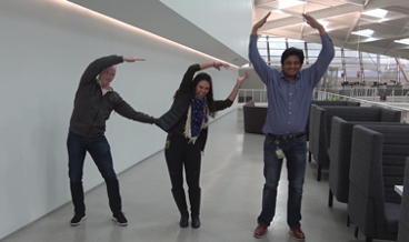
Figure 1 shows an example of the original image and Figure 2 shows the output image with pose results rendered. As you can see, the model is robust to an image that is different from the COCO training data.

Conclusion

In this post, you learned about training body pose models using the BodyPoseNet app in TLT. The post showed taking an open-source COCO dataset with a pretrained backbone from NGC to train a model with TLT. To optimize the trained model for inference and deployment, see Training and Optimizing the 2D Pose Estimation Model, Part 2.

For more information, see the following resources:

• Body Pose Estimation Training
• TLT Getting Started Guide
• Transfer Learning Toolkit
• TLT CV Inference Pipeline

The first post in this series covered how to train a 2D pose estimation model using an open-source COCO dataset with the BodyPoseNet app in the NVIDIA Transfer Learning Toolkit. In this post, you learn how to optimize the pose estimation model in the NVIDIA Transfer Learning Toolkit. It walks you through the steps of … Continued

The first post in this series covered how to train a 2D pose estimation model using an open-source COCO dataset with the BodyPoseNet app in the NVIDIA Transfer Learning Toolkit.

In this post, you learn how to optimize the pose estimation model in the NVIDIA Transfer Learning Toolkit. It walks you through the steps of model pruning and INT8 quantization to optimize the model for inference.

Model optimizations and export

This section covers few topics of model optimization and export:

• Pruning
• INT8 quantization
• Best practices for improving speed and accuracy

Pruning

BodyPoseNet supports model pruning to remove unnecessary connections, reducing the number of parameters by an order of magnitude. This results in an optimized model architecture.

Prune the model

To prune the model, use the following command:

tlt bpnet prune -m $USER_EXPERIMENT_DIR/models/exp_m1_unpruned/bpnet_model.tlt 
                 -o $USER_EXPERIMENT_DIR/models/exp_m1_pruned/bpnet_model.pruned-0.05.tlt 
                 -eq union 
                 -pth 0.05 
                 -k $KEY 

Usually, you just have to adjust -pth (threshold) for accuracy and model size trade off. For some internal studies, we’ve noticed that a pth value between the range [0.05, 3.0] is a good starting point for BodyPoseNet models.

Retrain the pruned model

After the model has been pruned, there might be a slight decrease in accuracy because some previously useful weights may have been removed. To regain the accuracy, we recommend retraining this pruned model over the same dataset. You can follow the same instructions as in the Train experiment configuration file section. The main change is now to specify pretrained_weights as the path to pruned model and enable load_graph. Because the model is being initialized with pruned model weights, the model converges faster.

# Retraining using the pruned model as model graph 
 tlt bpnet train -e $SPECS_DIR/bpnet_retrain_m1_coco.yaml 
                 -r $USER_EXPERIMENT_DIR/models/exp_m1_retrain 
                 -k $KEY 
                 --gpus $NUM_GPUS 

You can follow similar instructions as in the Evaluation and Model verification sections to evaluate and verify the pruned model. After retraining the pruned model with pth 0.05, you can observe an accuracy of 56.1% AP with multiscale inference. Here are the metrics on COCO validation set:

Average Precision  (AP) @[ IoU=0.50:0.95 | area=   all | maxDets= 20 ] = 0.561
Average Precision  (AP) @[ IoU=0.50      | area=   all | maxDets= 20 ] = 0.776
Average Precision  (AP) @[ IoU=0.75      | area=   all | maxDets= 20 ] = 0.609
Average Precision  (AP) @[ IoU=0.50:0.95 | area=medium | maxDets= 20 ] = 0.567
Average Precision  (AP) @[ IoU=0.50:0.95 | area= large | maxDets= 20 ] = 0.556
... 

Export the .etlt model

Inference throughput and how quickly you can create an efficient model are two key metrics for deploying deep learning applications because they directly affect the time to market and the cost of deployment. TLT includes an export command to export and prepare TLT models for deployment.

The model is exported as a .etlt (encrypted TLT) file. The file is consumable by the TLT CV Inference, which decrypts the model and converts it to a TensorRT engine. Exporting the model decouples the training process from inference and allows conversion to TensorRT engines outside the TLT environment. TensorRT engines are specific to each hardware configuration and should be generated for each unique inference environment. The following code example shows the export of the pruned, retrained model.

tlt bpnet export -m $USER_EXPERIMENT_DIR/models/exp_m1_retrain/bpnet_model.tlt 
                  -e $SPECS_DIR/bpnet_retrain_m1_coco.yaml 
                  -o $USER_EXPERIMENT_DIR/models/exp_m1_final/bpnet_model.etlt 
                  -k $KEY 
                  -t tfonnx 

The export command can optionally generate the calibration cache for running inference at INT8 precision. This is described more in detail in later sections.

INT8 quantization

The BodyPoseNet model supports int8 inference mode in TensorRT. To do this, the model is first calibrated to run 8-bit inferences. To calibrate the model, you need a directory with a sampled set of images to be used for calibration.

We’ve provided a helper script that parses the annotations and samples the required number of images at random based on specified criteria like number of people in the image, number of keypoints per person, and so on.

# Number of calibration samples to use
 export NUM_CALIB_SAMPLES=2000
  
 python3 sample_calibration_images.py 
     -a $LOCAL_EXPERIMENT_DIR/data/annotations/person_keypoints_train2017.json 
     -i $LOCAL_EXPERIMENT_DIR/data/train2017/ 
     -o $LOCAL_EXPERIMENT_DIR/data/calibration_samples/ 
     -n $NUM_CALIB_SAMPLES 
     -pth 1 
     --randomize 

Generate INT8 calibration cache and engine

The following command exports the pruned, retrained model to the .etlt format, performs INT8 calibration, and generates the INT8 calibration cache and TensorRT engine for the current hardware.

# Set dimensions of desired output model for inference/deployment
 export IN_HEIGHT=288
 export IN_WIDTH=384
 export IN_CHANNELS=3
 export INPUT_SHAPE=288x384x3
 # Set input name
 export INPUT_NAME=input_1:0
  
 tlt bpnet export 
     -m $USER_EXPERIMENT_DIR/models/exp_m1_retrain/bpnet_model.tlt 
     -o $USER_EXPERIMENT_DIR/models/exp_m1_final/bpnet_model.etlt 
     -k $KEY 
     -d $IN_HEIGHT,$IN_WIDTH,$IN_CHANNELS 
     -e $SPECS_DIR/bpnet_retrain_m1_coco.yaml 
     -t tfonnx 
     --data_type int8 
     --engine_file $USER_EXPERIMENT_DIR/models/exp_m1_final/bpnet_model.$IN_HEIGHT.$IN_WIDTH.int8.engine 
     --cal_image_dir $USER_EXPERIMENT_DIR/data/calibration_samples/ 
     --cal_cache_file $USER_EXPERIMENT_DIR/models/exp_m1_final/calibration.$IN_HEIGHT.$IN_WIDTH.bin  
     --cal_data_file $USER_EXPERIMENT_DIR/models/exp_m1_final/coco.$IN_HEIGHT.$IN_WIDTH.tensorfile 
     --batch_size 1 
     --batches $NUM_CALIB_SAMPLES 
     --max_batch_size 1 
     --data_format channels_last 

Make sure that the directory mentioned in --cal_image_dir has at least (batch_size * batches) number of images in it. To generate a F16 engine for the current hardware, specify --data_type as FP16. For more information about the parameters used here, see the INT8 model overview.

Evaluate the TensorRT engine

This evaluation is mainly used as a sanity check for the exported TRT (INT8/FP16) models. This doesn’t reflect the true accuracy of the model as the input aspect ratio here can vary a lot from the aspect ratio of the images in the validation set. The set has a collection of images with various resolutions. Here, you retain a strict input resolution and pad the image to retrain the aspect ratio. So, the accuracy here might vary based on the aspect ratio and the network resolution that you choose.

You can run the evaluation of the .tlt model in strict mode as well to compare with the accuracies of the INT8/FP16/FP32 models for any drop in accuracy. The FP16 and FP32 models should have no or minimal drop in accuracy when compared to the .tlt model in this step. The INT8 models would have similar accuracies (or comparable within 2-3% AP range) to the .tlt model.

You can follow similar instructions as in the Evaluation and Model verification sections to evaluate and verify the models. One change would be that you now use  $SPECS_DIR/infer_spec_retrained_strict.yaml as inference_spec and the model to use would be a pruned TLT model, INT8 engine, or FP16 engine.

Deployable model export

After the INT8/FP16/FP32 model is verified, you must reexport the model so it can be used to run on inference platforms like TLT CV Inference. You use the same guidelines as in the previous sections, but you must add the --sdk_compatible_model flag to the export command, which adds a few nontraininable post-process layers to the model to enable compatibility with the inference pipelines. Reuse the calibration tensorfile (cal_data_file) generated in the earlier step to keep it consistent, but you must regenerate the cal_cache_file and the .etlt model.

tlt bpnet export
     -m $USER_EXPERIMENT_DIR/models/exp_m1_retrain/bpnet_model.tlt
     -o $USER_EXPERIMENT_DIR/models/exp_m1_final/bpnet_model.deploy.etlt
     -k $KEY
     -d $IN_HEIGHT,$IN_WIDTH,$IN_CHANNELS
     -e $SPECS_DIR/bpnet_retrain_m1_coco.txt
     -t tfonnx
     --data_type int8
     --cal_image_dir $USER_EXPERIMENT_DIR/data/calibration_samples/
     --cal_cache_file $USER_EXPERIMENT_DIR/models/exp_m1_final/calibration.$IN_HEIGHT.$IN_WIDTH.deploy.bin
     --cal_data_file $USER_EXPERIMENT_DIR/models/exp_m1_final/coco.$IN_HEIGHT.$IN_WIDTH.tensorfile
     --batch_size 1
     --batches $NUM_CALIB_SAMPLES
     --max_batch_size 1
     --data_format channels_last
     --engine_file $USER_EXPERIMENT_DIR/models/exp_m1_final/bpnet_model.$IN_HEIGHT.$IN_WIDTH.int8.deploy.engine
     --sdk_compatible_model 

Best practices for improving speed and accuracy

In this section, we look at some best practices to improve model performance and accuracy.

Network input resolution for deployment

Network input resolution of the model is one of the major factors that determine the accuracy of bottom-up approaches. Bottom-up methods must feed the whole image at one time, resulting in a smaller resolution per person. Hence, higher input resolution yields better accuracy, especially on small- and medium-scale persons with regard to the image scale. However, with a higher input resolution, the runtime of the CNN also would be higher. So, the accuracy/runtime tradeoff should be determined by the accuracy and runtime requirements for the target use case.

If your application involves pose estimation for one or more persons close to the camera such that the scale of the person is relatively large, then you could go with a smaller network input height. If you are targeting to use the network for persons with smaller relative scales, like crowded scenes, you might want to go with a higher network input height. After you freeze the height of the network, the width can be decided based on the aspect ratio for your input data used during deployment time.

Illustration of accuracy/runtime variation for different resolutions

These are approximate runtimes and accuracies for the default architecture and spec used in the notebook. Any changes to the architecture or params yields different results. This is primarily to get a better sense of which resolution would suit your needs.

Input Resolution	Precision	Runtime (GeForce RTX 2080)	Runtime (Jetson AGX)
320×448	INT8	1.80ms	8.90ms
288×384	INT8	1.56ms	6.38ms
224×320	INT8	1.33ms	5.07ms

You can expect to see a 7-10% AP increase in the area=medium category when going from 224×320 to 288×384 and an additional 7-10% AP when you choose 320×448. The accuracy for area=large remains almost the same across these resolutions, so you can stick to a lower resolution if this is what you need. As per the COCO keypoint evaluation, medium area is defined as persons occupying less than area between 36^2 to 96^2. Anything higher is categorized as large.

We use a default size 288×384 in this post. To use a different resolution, you need the following changes:

• Update the env variables mentioned in INT8 quantization with the desired shape.
• Update the input_shape in infer_spec_retrained_strict.yaml, which enables you to do a sanity evaluation of the exported TRT model. By default, it is set to [288, 384].

The height and width should be a multiple of 8, preferably a multiple of 16/32/64.

Number of refinement stages in the network

Figure 1 shows that the model architecture includes refinement stages, where each stage refines the results of the previous stage. You can use the stages parameter under the model section to configure this. stages include both the initial prediction stage and the refinement stages. We recommend using a minimum of one refinement stage, and a maximum of six, which corresponds to stages within the range [2, 7].

When you use more stages of refinement, it may help improve the accuracy but keep in mind that this would result in an increased inference time. We use a default of two refinement stages (stages=3) in this post, which is tuned for optimal performance and accuracy. For even faster performance, use stages=2.

Pruning and regularization

Pruning can help with a significant decrease in the number of parameters and maximize speed while preserving the accuracy or at the cost of some drop in accuracy. A higher pruning threshold gives you a smaller model and thus higher inference speed but might cause a drop in accuracy.

The threshold to use depends on the dataset. If the retrain accuracy is good, you can increase this value to get smaller models. Otherwise, lower this value to get better accuracy. We recommend iterating with the prune-retrain cycle until you are satisfied with the accuracy-speed tradeoff. You can also use a higher L1 regularization weight when training the model before pruning. It would push more weights towards zero, making it easier to prune the network weights.

Model accuracy and performance

In this section, we dive deeper into the model accuracy and performance, and compare it against the state of the art, and across platforms.

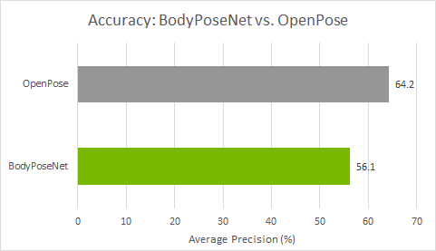
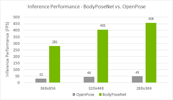
Comparison with OpenPose

We compare this approach against OpenPose as this method follows a similar single-shot bottom-up methodology. Figure 4 shows that you achieve a much better accuracy-performance tradeoff as compared to the OpenPose model. The accuracy is lower by ~8% AP whereas you achieve close to a 9x speedup for the model trained with the default parameters provided in this post.

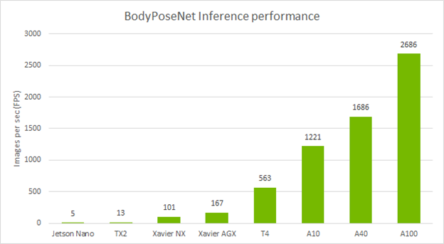
Standalone performance across devices

The following table shows the inference performance of the BodyPoseNet model trained with TLT by using the default parameters. We profiled the model inference with the trtexec command of TensorRT.

Conclusion

In this post, you learned about optimizing body pose models using the BodyPoseNet app in TLT. The post showed taking an open-source COCO dataset with a pretrained backbone from NGC to train and optimize a model with TLT. For information regarding model deployment, see the TLT CV inference pipeline Quick Start Scripts and Deployment instructions.

With this model, you can get up to 9x improvement in inference performance as compared to OpenPose, helping you achieve real-time performance even on embedded devices. Pruning plus INT8 precision gives you the highest inference performance on your edge devices.

For more information, see the following resources:

• Body Pose Estimation Training
• TLT Getting Started Guide
• Transfer Learning Toolkit
• TLT CV Inference Pipeline

It’s time for autonomous vehicle developers to blaze new trails.  NVIDIA has agreed to acquire DeepMap, a startup dedicated to building high-definition maps for autonomous vehicles to navigate the world safely.  “The acquisition is an endorsement of DeepMap’s unique vision, technology and people,” said Ali Kani, vice president and general manager of Automotive at NVIDIA. “DeepMap is expected to extend our mapping products, help us Read article >

The post NVIDIA to Acquire DeepMap, Enhancing Mapping Solutions for the AV Industry appeared first on The Official NVIDIA Blog.

submitted by /u/slowkevin
[visit reddit] [comments]