Accelerating Blender Python Using CUDA

Simulated or synthetic data generation is an important emerging trend in the development of AI tools. Classically, these datasets can be used to address low-data problems or edge-case scenarios that might now be present in available real-world datasets. Emerging applications for synthetic data include establishing model performance levels, quantifying the domain of applicability, and next-generation … Continued

Emerging applications for synthetic data include establishing model performance levels, quantifying the domain of applicability, and next-generation systems engineering, where AI models and sensors are designed in tandem.

Picture of a ship next a representation of the ship’s phase map, which is composed of lines and colors. — *Figure 1.* *Synthetic SAR render of a ship: Phase map (*left), Compressed image (right).

Blender is a common and compelling tool for generating these datasets. It is free to use and open source but, just as important, it is fully extensible through a powerful Python API. This feature of Blender has made it an attractive option for visual image rendering. As a result, it has been used extensively for this purpose, with 18+ rendering engine options to choose from.

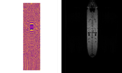
Rendering engines integrated into Blender, such as Cycles, often come with tightly integrated GPU support, including state-of-the-art NVIDIA RTX support. However, if high performance levels are required outside of a visual rendering engine, such as the render of a synthetic SAR image, the Python environment can be too sluggish for practical applications. One option to accelerate this code is to use the popular Numba package to precompile portions of the Python code into C. This still leaves room for improvement, however, particularly when it comes to the adoption of leading GPU architectures for scientific computing.

GPU capabilities for scientific computing can be available from directly within Blender, allowing for simple unified tools that leverage Blender’s powerful geometry creation capabilities as well as cutting-edge computing environments. As of the recent changes in Blender 2.83+, this can be done using CuPy, a GPU-accelerated Python library devoted to array calculations, directly from within a Python script.

In line with these ideas, the following tutorial compares two different ways of accelerating matrix multiplication. The first approach uses Python’s Numba compiler while the second approach uses the NVIDIA GPU-compute API, CUDA. Implementation of these approaches can be found in the rleonard1224/matmul GitHub repo, along with a Dockerfile that sets up an anaconda environment from which CUDA-accelerated Blender Python scripts can be run.

Matrix multiplication algorithms

As a precursor to discussing the different approaches used to accelerate matrix multiplication, we briefly review matrix multiplication itself.

For the product of two matrices $[A cdot B]$ to be well defined, the number of columns of $[A]$ must be equal to the number of rows of $[B]$ .

$[A]$ then is a matrix with $[m]$ rows and $[n]$ columns, that is, an $[m times n]$ matrix.
$[B]$ is an $[n times p]$ matrix.
The product $[C = A cdot B]$ results in an $[m times p]$ matrix.

If the first element in each row and each column of $[C]$ , $[A]$ , and $[B]$ are indexed with the number one—that is, one-based indexing, then the element in the i-th row and j-th column of $[C]$ , $[C[i,j]]$ , is determined by the following formula:

$[C[i,j] = Sigma_{r = 1}^{n} A[i,r] cdot B[r,j]]$

Numba acceleration

The Numba compiler can be applied to a function in a Python script by using the numba.jit decorator. By precompilation into C, the use of the numba.jit decorator significantly reduces the run times of loops when used in Python code. Because matrix multiplication translated directly into code requires nested for loops, use of the numba.jit decorator significantly reduces the run times of a matrix multiplication function written in Python. The matmulnumba.py Python script implements matrix multiplication and uses the numba.jit decorator.

CUDA acceleration

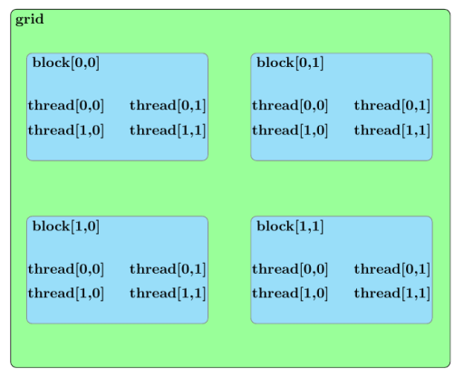
Before we discuss an approach to accelerate matrix multiplication using CUDA, we should broadly outline the parallel structure of a CUDA kernel launch. All parallel processes within a kernel launch belong to a grid. A grid is composed of an array of blocks and each block is composed of an array of threads. The threads within a grid compose the fundamental parallel processes launched by a CUDA kernel. Figure 2 outlines a sample parallel structure of this kind.

Picture of a grid arranged as a 2x2 matrix representing a CUDA kernel grid with each element of the matrix representing a CUDA block. — *Figure 2.* *Parallel structure of a CUDA kernel grid composed of a 2×2 array of blocks. Each block is composed of a 2×2 array of threads.*

Now that this summary of the parallel structure of a CUDA kernel launch is spelled out, the approach used to parallelize matrix multiplication in the matmulcuda.py Python script can be described as follows.

Suppose the following are to be calculated by a CUDA kernel grid composed of a 2D array of blocks with each block composed of a 1D array of threads:

matrix product
- $[A]$ and $[m times n]$ matrix
- $[B]$ and $[n times p]$ matrix
- $[C]$ and $[m times p]$ matrix

Also, further assume the following:

The number of blocks in the x-dimension of the grid ( $[textrm{nblocksx}]$ ) is greater than or equal to $[m]$ ( $[textrm{nblocksx} geq m]$ ).
The number of blocks in the y-dimension of the grid ( $[textrm{nblocksy}]$ ) is greater than or equal to $[p]$ ( $[textrm{nblocksy} geq p]$ ).,
The number of threads in each block ( $[textrm{nthreads}]$ ) is greater than or equal to $[n]$ ( $[textrm{nthreads} geq n]$ ).

The elements of the matrix product $[C = A cdot B]$ can be calculated in parallel by assigning to each block the calculation of an element of $[C]$ , $[C[i,j]]$ .

You can obtain further parallel enhancement by assigning, to each thread of the block to which $[C[i,j]]$ was assigned, the calculation of one of the $[n]$ products whose sum equals $[C[i,j]]$ .

To avoid a race condition, the summing of these $[n]$ products and the assignment of the result to $[C[i,j]]$ can be handled using the CUDA atomicAdd function. The atomicAdd function signature consists of a pointer as the first input and a numerical value as the second input. The definition adds the numerical value input to the value pointed to by the first input and later stores this sum in the location pointed to by the first input.

Assume that the elements of $[C]$ are initialized to zero and that $[textrm{tid}(i,j)]$ denoting the thread index of a thread belonging to a block with indices in the grid of $[[i,j]]$ . The preceding parallel arrangement can be summarized by the following equation:

$[C[i,j] = textrm{atomicAdd}(C[i,j], A[i, textrm{tid}(i,j)] cdot B[textrm{tid}(i,j), j])]$

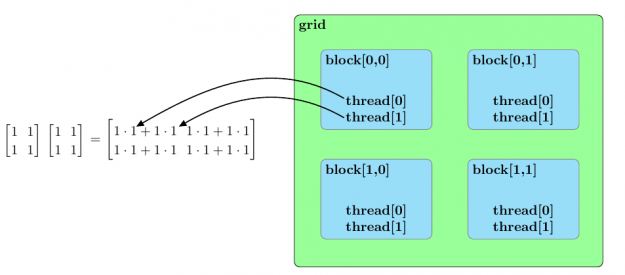
Figure 3 summarizes this parallel arrangement for the multiplication of two sample matrices of $[2 times 2]$ .

Grid composed of blocks in a 2x2 grid, which parallelize the multiplication of two 2x2 matrices composed of ones. — Figure 3. A way to parallelize the multiplication of two 2×2 matrices. Each block is assigned one element of the product of the two matrices and the threads in a thread block parallelize the calculation of the products necessary to determine the value of the matrix element to which the block is assigned.

Speedups

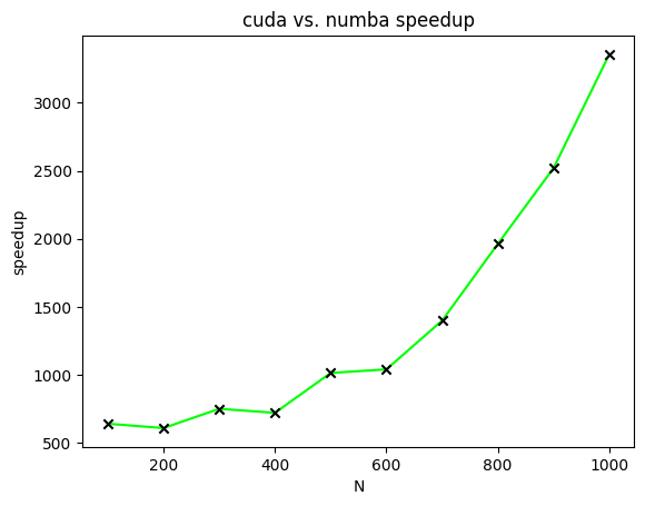
Figure 4 displays the speedups of CUDA-accelerated matrix multiplication relative to Numba-accelerated matrix multiplication for matrices of varying sizes. In this figure, speedups are plotted for the calculation of two $[N times N]$ matrices with all elements of both matrices equal to one. $[N]$ ranges from one hundred to one thousand in increments of one hundred.

One-dimensional plot showing increasing speedup of CUDA relative to Numba as the size of the matrices increases. — *Figure 4. Speedup of cuda-accelerated matrix multiplication relative to Numba-accelerated matrix multiplication for the multiplication of two NxN matrices.*

Future work

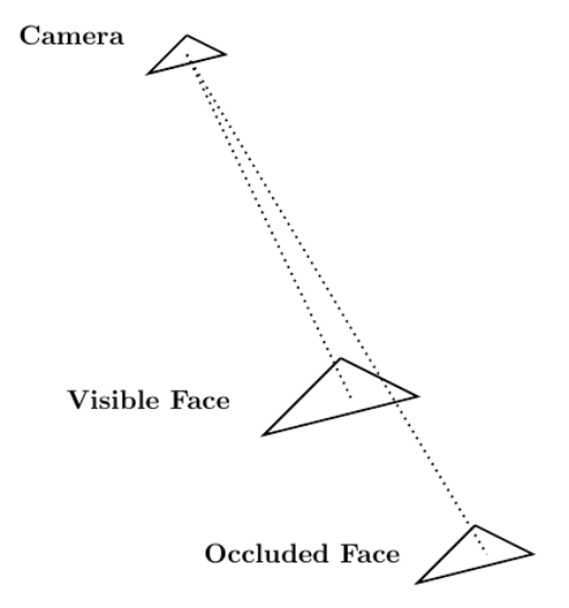
Given Blender’s role as a computer graphics tool, one relevant area of application suitable for CUDA acceleration relates to solving the visibility problem through ray tracing. The visibility problem can be broadly summarized as follows: A camera exists at some point in space and is looking at a mesh composed of, for instance, triangular elements. The goal of the visibility problem is to determine which mesh elements are visible to the camera and which are instead occluded by other mesh elements.

Ray tracing can be used to solve the visibility problem. A mesh whose visibility you are trying to determine is composed of $[N]$ mesh elements. In that case, $[N]$ rays can be generated whose origin point is the camera in the scene. Those endpoints are located at the center of the $[N]$ mesh elements.

Each ray has an endpoint at a different mesh element. If a ray reaches its endpoint without being occluded by another mesh element, then the endpoint mesh element is visible from the camera. Figure 5 shows this procedure.

One face blocking another face from the viewpoint of a camera. — Figure 5. *Two rays emanating from a camera toward the faces in the scene; one face is visible while the other is occluded.*

The nature of the use of ray tracing to solve the visibility problem makes it an $[mathcal{O}(N^{2})]$ problem when implemented as a direct calculation. Fortunately, NVIDIA has developed a ray tracing library, named NVIDIA OptiX, which uses GPU parallelism to achieve significant speedups. Use of NVIDIA OptiX from within a Blender Python environment would then offer tangible benefits.

Summary

This post described two different approaches for how to accelerate matrix multiplication. The first approach used the Numba compiler to decrease the overhead associated with loops in Python code. The second approach used CUDA to parallelize matrix multiplication. A speed comparison demonstrated the effectiveness of CUDA in accelerating matrix multiplication.

Because the CUDA-accelerated code described earlier can be run as a Blender Python script, any number of algorithms can be accelerated using CUDA from within a Blender Python environment. That greatly increases the effectiveness of Blender Python as a scientific computing tool.

If you have questions or comments, please comment below or contact us at info@rendered.ai.