
 Connected cars are vehicles that communicate with other vehicles using backend systems to enhance usability, enable convenient services, and keep distributed software maintained and up to date. At Volkswagen, we are working on connected car with NVIDIA to solve the challenges which have computational inefficiencies like Geospatial Indexing and K-Nearest Neighbors when implemented in native … Continued
Connected cars are vehicles that communicate with other vehicles using backend systems to enhance usability, enable convenient services, and keep distributed software maintained and up to date.
At Volkswagen, we are working on connected car with NVIDIA to solve the challenges which have computational inefficiencies like Geospatial Indexing and K-Nearest Neighbors when implemented in native python and pandas.
Processing driving and sensor data is critical for connected cars to understand their environment. It enables connected cars to perform tasks such as parking spot detection, location-based services, theft protection, route recommendation through real-time traffic, fleet management, and many more. Location information is key to most of these use cases and requires a fast processing pipeline to enable real-time services.
Global sales of connected cars are increasing rapidly, in turn, increasing the amount of data available. As per Gartner, the average connected vehicle will generate 280 petabytes of data annually, with four terabytes of data being generated in a day at the very least. The research also states that around 470 million connected vehicles will be deployed by 2025.
This blog post will focus on the data pipeline required to process location-based geospatial information and deliver necessary services for connected cars.
Challenges with connected cars data
Working with connected car data poses both technical and business challenges:
Fast processing of huge amounts of streaming data is needed because users expect a near real-time experience to make timely decisions. For example, if a user requests a parking spot and the system takes five minutes to respond, it’s likely the spot will already be taken by the time it answers. Faster processing and analyzing of the data is the key factor to overcome this challenge.
There are also data privacy issues to consider. Connected cars must satisfy the General Data Protection Regulation (GDPR). In short, GDPR requires that after data analysis, there should not be a chance to identify individual users from the analyzed data. Additionally, storage of data pertaining to individual users is prohibited (unless written consent is given by the user). Anonymization can meet these requirements by either masking the data that identifies the individual user or by grouping and aggregating the data so that traces of the user are not possible. For this purpose, we need to make sure that the software processing connected car data complies with the regulations required by GDPR on data anonymization, which adds additional compute requirements during the data processing.

Taking a data science approach
RAPIDS can address both the technical and business challenges of connected cars. The RAPIDS suite of open-source software (OSS) libraries and APIs gives you the ability to execute end-to-end data science and analytics pipelines entirely on GPUs. Licensed under Apache 2.0, RAPIDS was incubated by NVIDIA and based on extensive hardware and data science experience. RAPIDS utilizes NVIDIA CUDA primitives for low-level compute optimization and exposes GPU parallelism and high-bandwidth memory speed through user-friendly Python interfaces.
In the following sections, we discuss how RAPIDS (software) and NVIDIA GPUs (hardware) help tackle both the technical and business challenges on a prototype application using test data. Two different approaches will be evaluated, geospatial indexing and k-nearest neighbors.
Using RAPIDS, we are able to achieve a 100x speedup for this pipeline.
A brief introduction to geospatial indexing
Geospatial indexing is the basis for many algorithms in the domain of connected cars. It is the process of partitioning areas of the earth into identifiable grid cells. It is an effective way to prune the search space when querying the huge amount of data produced by connected cars.
Popular approaches include Military Grid Reference System (MGRS) and Uber’s Hexagonal Hierarchical Spatial Index (Uber H3).
In this data pipeline example, we use Uber H3 to split the records spatially into a set of smaller subsets.
The following are the conditions, which need to be satisfied after splitting the records into subsets:
- Each subset consists of a maximum of ‘N’ records. This ‘N’ is chosen based on computational capacity constraints. For this experiment, we consider ‘N’ equals 2500 records.
- The subset is denoted by subset_id, which is an auto-increment number starting from 0.
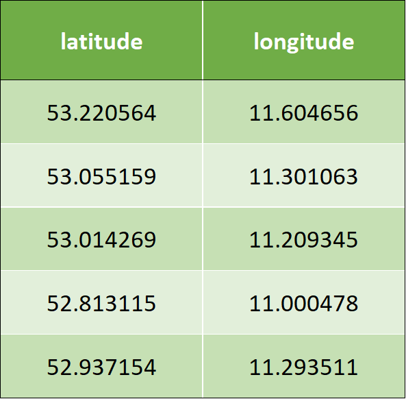
The following is the sample input data, which has two columns – latitude and longitude:
The following is the algorithm that needs to be implemented to apply Uber H3 for the use case
- Iterate over latitude and longitude, and assign hex_id from resolution 0.
- If found any hex_id comprising less than 2500 records, then assign subset_id incrementally starting from 0.
- Identify the hex_ids that comprise more than 2500 records.
- Split the preceding records with an incremental resolution, which is now 1.
- Repeat steps 3 and 4, until all the records are assigned to subset_id & hex_id or until the resolution reaches 15.
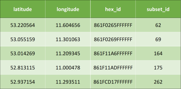
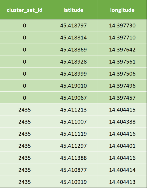
Once the preceding algorithm is applied, it results to the following output data:
Code snippets of Uber H3 implementation
Following is the code snippet of the implementation of Uber H3 using pandas:
#while loop until all the records are assigned to subset_id
while resolution  16 and df["subset_id"].isnull().any():
     #assignment of hex_id
     df['hex_id']= df.apply(lambda row: h3.geo_to_h3(row["latitude"],
                   row["longitude"], resolution), axis = 1)
      df_aggreg = df.groupby(by = "hex_id").size().reset_index()
     df_aggreg.columns = ["hex_id", "value"]
      #filtering the records that are less than 2500 count
     hex_id = df_aggreg[df_aggreg['value']2500]['hex_id']
      #assignment of subset_id
     for index, value in hex_id.items():
         df.loc[df['hex_id'] == value, 'subset_id'] = subset_id
         subset_id += 1
     df_return = df_return.append(df[~df['subset_id'].isna()],
                 ignore_index=True)
     df = df[df['subset_id'].isna()]
     resolution += 1
Following is the code snippet of the implementation of Uber H3 using PySpark:
#while loop until all the records are assigned to subset_id
while resolution  16 and (len(df.head(1)) != 0):
      #assignment of hex_id
     df = df.rdd.map(lambda x: (x["latitude"], x["longitude"],
          x["subset_id"],h3.geo_to_h3(x["latitude"], x["longitude"],
          resolution)))
      df = sqlContext.createDataFrame(df, schema)
     df_aggreg = df.groupby("hex_id").count()
     df_aggreg = df_aggreg.withColumnRenamed("hex_id", "hex_id")
          .withColumnRenamed("count", "value")
      #filtering the records that are less than 2500 count
     hex_id = df_aggreg.filter(df_aggreg.value  2500)
     var_hex_id = list(hex_id.select('hex_id').toPandas()['hex_id'])
     for i in var_hex_id:
         #assignment of subset_id
         df = df.withColumn('subset_id',F.when(df.hex_id==i,subset_id)
             .otherwise(df.subset_id)).select(df.latitude, df.longitude,
             'subset_id', df.hex_id)
          subset_id += 1
      df_return = df_return.union(df.filter(df.subset_id != 0))
     df = df.filter(df.subset_id == 0)
     resolution += 1
With this pandas implementation of the Uber H3 model, we have identified a painfully slow execution. The slow execution of the code leads to significantly reduced productivity, as only little experiments can be done. The tangible goal is to speed up the execution time by 10x.
To accelerate the pipeline, we follow a step-by-step approach as follows.
Step 1: Simple CPU parallel version
The idea of this version is to implement a simple multiprocessing-based kernel for the H3 library processing. The second part of the processing, which is assigning subsets according to the data, is the pandas library function, which cannot be easily parallelized.
#Function to assign hex_id
def minikernel(df, resolution):
 df['hex_id'] = np.vectorize(lambda latitude, longitude:
                 h3.geo_to_h3(latitude, longitude, resolution))(
                 np.array(df['latitude']), np.array(df['longitude']))
  return df
#while loop until all the records are assigned to subset_id
while resolution  16 and df["subset_id"].isnull().any():
     #CPU Parallelization
     df_chunk = np.array_split(df, n_cores)
     pool = Pool(n_cores)

     #assigning hex_id by calling the function minikernel()
     df_chunk_res=pool.map(partial(minikernel, resolution=resolution),
                     df_chunk)

     df = pd.concat(df_chunk_res)

     pool.close()
     pool.join()

     df_aggreg = df.groupby(by = "hex_id").size().reset_index()
     df_aggreg.columns = ["hex_id", "value"]

     #filtering the records that are less than 2500 count
     hex_id = df_aggreg[df_aggreg['value']2500]['hex_id']

     for index, value in hex_id.items():
            #assignment of subset_id is pandas library function
            #which cannot be parallelized
         df.loc[df['hex_id'] == value, 'subset_id'] = subset_id
         subset_id += 1

     df_return = df_return.append(df[~df['subset_id'].isna()],
                 ignore_index=True)

     df = df[df['subset_id'].isna()]
     resolution += 1
By applying simple parallelization with a thread pool, we can significantly reduce the first part of the code (H3 library), but the second part (pandas library) is completely single-threaded and extremely slow.
Step 2: Apply RAPIDS cuDF
The idea here is to use as many standard features from cuDF as possible (hence, the slightest code change) to achieve the best performance. As cuDF now operates on CUDA unified memory, it is not simply possible to parallelize the 1st part (H3 library) as cuDF does not handle CPU partitioning. The code is shown below. Note, the following code operates on a cuDF dataframe.
#while loop until all the records are assigned to subset_id
while resolution  16 and df["subset_id"].isnull().any():
     #assignment of hex_id
     #df is a cuDF
     df['hex_id'] = np.vectorize(lambda latitude, longitude:
                     h3.geo_to_h3(latitude, longitude, resolution))
                     (df['latitude'].to_array(), df['longitude']
                     .to_array())

     df_aggreg = df.groupby('hex_id').size().reset_index()
     df_aggreg.columns = ["hex_id", "value"]

     #filtering the records that are less than 2500 count
     hex_id = df_aggreg[df_aggreg['value']2500]['hex_id']

     for index, value in hex_id.to_pandas().items():
         #assignment of subset_id
         df.loc[df['hex_id'] == value, 'subset_id'] = subset_id
         subset_id += 1

     df_return = df_return.append(df[~df['subset_id'].isna()],
                 ignore_index=True)

     df = df[df['subset_id'].isna()]

     resolution += 1
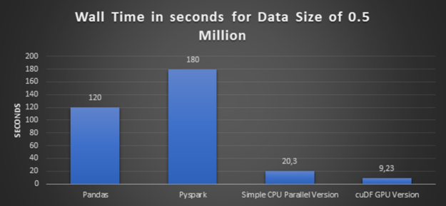
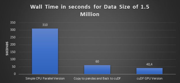
Step 3: Executing simple CPU parallelism version and cuDF GPU version using larger data
In this step, we increase the data volume three times, from half a million records to 1.5 million records, and execute a simple CPU parallel version and its equivalent cuDF GPU version.
Step 4: One more experiment with a copy to pandas and back to cuDF
As discussed in step 2, cuDF operates on CUDA-unified memory and it is not possible to parallelize the first part (H3 library) due to the lack of CPU-partitioning of the cuDF. Therefore, we have not used the function array_split. To overcome this challenge, first, we converted cuDF to pandas data frame, then applied the function array_split and then converted back the split chunk to cuDF and proceeded further with H3 library processing.
#while loop until all the records are assigned to subset_id
while resolution  16 and df["subset_id"].isnull().any():
     #copy to pandas
     df_temp = df.to_pandas()

     #CPU Parallelization
     df_chunk = np.array_split(df_temp, n_cores)
     pool = Pool(n_cores)
     df_chunk_res=pool.map(partial(minikernel, resolution=resolution),
                     df_chunk)

     pool.close()
     pool.join()

     df_temp = pd.concat(df_chunk_res)

     #Back to cuDF
     df = cudf.DataFrame(df_temp)

     #assignment of hex_id
     df['hex_id'] = np.vectorize(lambda latitude, longitude:
                     h3.geo_to_h3(latitude, longitude, resolution))
                     (df['latitude'].to_array(), df['longitude']
                     .to_array())

     df_aggreg = df.groupby('hex_id').size().reset_index()
     df_aggreg.columns = ["hex_id", "value"]

     #filtering the records that are less than 2500 count
     hex_id = df_aggreg[df_aggreg['value']2500]['hex_id']

     for index, value in hex_id.to_pandas().items():
         #assignment of subset_id
         df.loc[df['hex_id'] == value, 'subset_id'] = subset_id
         subset_id += 1

     df_return = df_return.append(df[~df['subset_id'].isna()],
                 ignore_index=True)

     df = df[df['subset_id'].isna()]

     resolution += 1
Glancing graph with execution times over all the preceding approaches:
Lessons learned on speed-up geospatial index computation
- High-Performance: The conclusion from the preceding glancing graphs is clear that cuDF GPU version delivers the best performance. And also bigger the dataset is, bigger the speedup is.
- Code Adaptability and Easy Transition: Please notice that the code being ported is not the best scenario for GPU acceleration. We are running the comparison on a third-party library (Uber H3) which runs on CPU. To make use of that library, we need to copy the data from GPU memory to CPU memory on each loop, which is not the optimal approach.
In addition to that, there is a subset_id calculation that is also done in a row-wise approach, which could potentially be speeded up by changing the original code. But still, the code is not changed because one of our main targets is to check code adaptability and easy transition between the libraries pandas and cuDF. - Reusable Code: As you had already observed from the preceding that the pipeline is a set of standardized functions and can just be used as functions to solve other use cases too.
Working towards a CUDA accelerated K-Nearest Neighbors (KNN) classification
Rather than measuring the density of connected cars by means of indexing and grouping, using the scheme above – another way is to perform geographical classification based on the earth distance between two locations.
The classification algorithm of our choice is K-Nearest Neighbors. The principle behind nearest neighbor methods is to find a predefined number of data points (K) closest in distance to the data point. We will be comparing a CPU-based implementation of KNN to the RAPIDS GPU-accelerated version of the same algorithm.
In our current use case, we work with anonymized streamed connected car data (as shortly described in business challenges preceding). Here, grouping and aggregating data using KNN is opted as part of anonymization.
However, for our use case, as we are grouping and aggregating on Geo-Coordinates, we will be using Haversine metric, which is the only metric that can cluster Geo-Coordinates.
In our pipeline inputs to KNN using haversine as distance metric will be the geo-coordinates (latitude, longitude) and the number of desired closest data points. In the example below, K = 7 was to be created.
In the following, we showcase the example with the same data in tuples (longitude and latitude).
- Input data are the same tuples (longitude and latitude) as shown in the previous example.
- Once KNN is applied, a cluster id is calculated by the KNN algorithm: The clustered output data looks like below for the first two rows of input data. To avoid confusion, we marked the cluster ids with corresponding colors.
Following is the code snippet of the implementation of KNN using pandas:
nbrs = NearestNeighbors(n_neighbors=7, algorithm='ball_tree',
     metric = "haversine").fit(coord_array_rad)

distances, indices = nbrs.kneighbors(coord_array_rad)

# Distance is computed in radians from haversine
distances_m = earth_radius * distances

# Drop KNN, which are not compliant with minimum distance
compliant_distances_mask = (distances_mKNN_MAX_DISTANCE)
                         .all(axis = 1)

compliant_indices = indices[compliant_distances_mask]
KNN is used as a classification algorithm. Drawback of KNN is its computational performance, especially when the data size is large. Our intention is to finally leverage cuML´s KNN implementation.
Preceding implementation worked in pretty small datasets but did not finish processing 3 million records within 1.5 days. Thus we stopped it.
In order to turn towards the CUDA accelerated KNN implementation, we had to mimic the haversine distance with an equivalent metric as shown below.
Step 1: Coordinate transformation to work around Haversine
At the moment of running this exercise, haversine distance metric was not available natively in cuML’s KNN implementation. Therefore, euclidean distance was used instead. Nevertheless, it is fair to mention that the current version of RAPIDS KNN already supports haversine metrics.
First of all, we converted the coordinates into the distance in meters in order to perform a distancing metric calculation. [10] This is implemented through a function named df_geo(), which will be used in the next step.
One caveat of Euclidean distance is that it does not work on coordinates on earth that are further distanced. Rather, it will basically “dig a hole” into the earth’s surface instead of being on the surface of the earth. However, for smaller distances
Step 2: Perform KNN algorithm
By now, we have converted all coordinates into a north-easting coordinate format and in this step, the actual KNN algorithm can be applied.
We used the CUDA accelerated KNN in the following setting. We observe that this implementation performs extremely fast and it is absolutely worthy implementation.
#defining the hyperparameters
n_neighbors = 7
algorithm = "brute"
metric = "euclidean"

#Implementation of kNN by calling df_geo() which converts the coordinates #into Northing and Easting coordinate format
nbrs = NearestNeighbors(n_neighbors=n_neighbors, algorithm=algorithm,
     metric=metric).fit(df_geo[['northing', 'easting']])

distances, indices = nbrs.kneighbors(df_geo[['northing', 'easting']])
Step 3: Perform the distance masking and filtering
This part is done on the CPU again because no significant speedup is expected on the GPU.
distances = cp.asnumpy(distances.values)
indices = cp.asnumpy(indices.values)
#running on CPU
KNN_MAX_DISTANCE = 10000 # meters

# Drop KNN, which are not compliant with minimum distance
compliant_distances_mask = (distances  KNN_MAX_DISTANCE).all(axis = 1)
compliant_indices = indices[compliant_distances_mask]
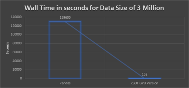
Our result is a speedup of 800x when applied to a dataset with 3 million samples over the naive pandas implementation.
Lessons learnt for K-Nearest Neighbors (KNN) clustering
- High-Performance: The conclusion from the preceding glancing graph is clear that, cuDF GPU version delivers the best performance. Even though the dataset is bigger, the execution will not take a long time like in CPU executions.
- Comparing KNN from cuML and scikit: The cuML based implementation is lightning fast. But we had to go the extra mile to mimic the missing distance metric. It was absolutely worth doing more than required given the performance boost achieved. In the meantime, the haversine distance is supported in RapidsAI and comes at the same convenience as the scikit implementation.
We overcome the missing haversine distance by using the Euclidean distance with Northing-Easting Approach. As per the research “Over fairly large distances–perhaps up to a few thousand kilometers or more, Euclidean starts erroneous calculation” In our code, we are limiting the distance to 10 Kilometers. By using Northing-Easting, we first needed to convert the coordinates. As the overall performance is much better, we can accept the time taken for converting the coordinates. - Code Adaptability and Easy Transition: Except the Northing-Easting function.
- The remaining code is similar to CPU code and still achieved better performance. We had not changed the code because one of our main targets is also to check code adaptability and easy transition between the libraries pandas and cuDF.
- Reusable Code: As you already observed from the preceding, pipeline is a set of standardized functions and can be used as functions to solve other use cases too.
Summary
This article summarized how RAPIDS helps in accelerating data pipelines 100x faster by evaluating it over two models, namely Geospatial Indexing (Uber H3) and K-Nearest Neighbors Classification (KNN). Furthermore, we analyzed the advantages and disadvantages of NVIDIA RapidsAI with respect to the preceding two models with many criteria like performance, code adaptability, and reusability. We conclude that RAPIDS is surely a technology for streaming data processing (connected car data). It provides the benefits of faster processing of data which is the crucial factor for streaming data analysis. Also, RAPIDS has a large number of machine learning algorithms supported. The API’s of accelerated RAPIDS cuDF and cuML libraries kept similar to pandas to enable the easy transition. It is very easy to transform existing ML pipelines and make them benefit from cuDF and cuML.
When to choose RAPIDS over standard Python and pandas:
- When the application requires faster processing of data.
- If you are sure that the code gives benefits on running in GPU over CPU.
- If the recommended algorithms are available as part of cuML.
This article aims at automotive engineers, data engineers, big data architects, project managers, and industry consultants interested in exploring or dealing with the possibilities of data science and using Python to analyze data.
- Listen to the GTC session: Accelerating VW Connected-Car Data Pipelines 100x Faster with RAPIDS [E31421]