
Month: July 2021
Natural image synthesis is a broad class of machine learning (ML) tasks with wide-ranging applications that pose a number of design challenges. One example is image super-resolution, in which a model is trained to transform a low resolution image into a detailed high resolution image (e.g., RAISR). Super-resolution has many applications that can range from restoring old family portraits to improving medical imaging systems. Another such image synthesis task is class-conditional image generation, in which a model is trained to generate a sample image from an input class label. The resulting generated sample images can be used to improve performance of downstream models for image classification, segmentation, and more.
Generally, these image synthesis tasks are performed by deep generative models, such as GANs, VAEs, and autoregressive models. Yet each of these generative models has its downsides when trained to synthesize high quality samples on difficult, high resolution datasets. For example, GANs often suffer from unstable training and mode collapse, and autoregressive models typically suffer from slow synthesis speed.
Alternatively, diffusion models, originally proposed in 2015, have seen a recent revival in interest due to their training stability and their promising sample quality results on image and audio generation. Thus, they offer potentially favorable trade-offs compared to other types of deep generative models. Diffusion models work by corrupting the training data by progressively adding Gaussian noise, slowly wiping out details in the data until it becomes pure noise, and then training a neural network to reverse this corruption process. Running this reversed corruption process synthesizes data from pure noise by gradually denoising it until a clean sample is produced. This synthesis procedure can be interpreted as an optimization algorithm that follows the gradient of the data density to produce likely samples.
Today we present two connected approaches that push the boundaries of the image synthesis quality for diffusion models — Super-Resolution via Repeated Refinements (SR3) and a model for class-conditioned synthesis, called Cascaded Diffusion Models (CDM). We show that by scaling up diffusion models and with carefully selected data augmentation techniques, we can outperform existing approaches. Specifically, SR3 attains strong image super-resolution results that surpass GANs in human evaluations. CDM generates high fidelity ImageNet samples that surpass BigGAN-deep and VQ-VAE2 on both FID score and Classification Accuracy Score by a large margin.
SR3: Image Super-Resolution
SR3 is a super-resolution diffusion model that takes as input a low-resolution image, and builds a corresponding high resolution image from pure noise. The model is trained on an image corruption process in which noise is progressively added to a high-resolution image until only pure noise remains. It then learns to reverse this process, beginning from pure noise and progressively removing noise to reach a target distribution through the guidance of the input low-resolution image..
<!– –>
With large scale training, SR3 achieves strong benchmark results on the super-resolution task for face and natural images when scaling to resolutions 4x–8x that of the input low-resolution image. These super-resolution models can further be cascaded together to increase the effective super-resolution scale factor, e.g., stacking a 64×64 → 256×256 and a 256×256 → 1024×1024 face super-resolution model together in order to perform a 64×64 → 1024×1024 super-resolution task.
We compare SR3 with existing methods using human evaluation study. We conduct a Two-Alternative Forced Choice Experiment where subjects are asked to choose between the reference high resolution image, and the model output when asked the question, “Which image would you guess is from a camera?” We measure the performance of the model through confusion rates (% of time raters choose the model outputs over reference images, where a perfect algorithm would achieve a 50% confusion rate). The results of this study are shown in the figure below.
 |
| Above: We achieve close to 50% confusion rate on the task of 16×16 → 128×128 faces, outperforming state-of-the-art face super-resolution methods PULSE and FSRGAN. Below: We also achieve a 40% confusion rate on the much more difficult task of 64×64 → 256×256 natural images, outperforming the regression baseline by a large margin. |
CDM: Class-Conditional ImageNet Generation
Having shown the effectiveness of SR3 in performing natural image super-resolution, we go a step further and use these SR3 models for class-conditional image generation. CDM is a class-conditional diffusion model trained on ImageNet data to generate high-resolution natural images. Since ImageNet is a difficult, high-entropy dataset, we built CDM as a cascade of multiple diffusion models. This cascade approach involves chaining together multiple generative models over several spatial resolutions: one diffusion model that generates data at a low resolution, followed by a sequence of SR3 super-resolution diffusion models that gradually increase the resolution of the generated image to the highest resolution. It is well known that cascading improves quality and training speed for high resolution data, as shown by previous studies (for example in autoregressive models and VQ-VAE-2) and in concurrent work for diffusion models. As demonstrated by our quantitative results below, CDM further highlights the effectiveness of cascading in diffusion models for sample quality and usefulness in downstream tasks, such as image classification.
 |
| Example of the cascading pipeline that includes a sequence of diffusion models: the first generates a low resolution image, and the rest perform upsampling to the final high resolution image. Here the pipeline is for class-conditional ImageNet generation, which begins with a class-conditional diffusion model at 32×32 resolution, followed by 2x and 4x class-conditional super-resolution using SR3. |
 |
| Selected generated images from our 256×256 cascaded class-conditional ImageNet model. |
Along with including the SR3 model in the cascading pipeline, we also introduce a new data augmentation technique, which we call conditioning augmentation, that further improves the sample quality results of CDM. While the super-resolution models in CDM are trained on original images from the dataset, during generation they need to perform super-resolution on the images generated by a low-resolution base model, which may not be of sufficiently high quality in comparison to the original images. This leads to a train-test mismatch for the super-resolution models. Conditioning augmentation refers to applying data augmentation to the low-resolution input image of each super-resolution model in the cascading pipeline. These augmentations, which in our case include Gaussian noise and Gaussian blur, prevents each super-resolution model from overfitting to its lower resolution conditioning input, eventually leading to better higher resolution sample quality for CDM.
Altogether, CDM generates high fidelity samples superior to BigGAN-deep and VQ-VAE-2 in terms of both FID score and Classification Accuracy Score on class-conditional ImageNet generation. CDM is a pure generative model that does not use a classifier to boost sample quality, unlike other models such as ADM and VQ-VAE-2. See below for quantitative results on sample quality.
 |
| Class-conditional ImageNet FID scores at the 256×256 resolution for methods that do not use extra classifiers to boost sample quality. BigGAN-deep is reported at its best truncation value. (Lower is better.) |
 |
| ImageNet classification accuracy scores at the 256×256 resolution, measuring the validation set accuracy of a classifier trained on generated data. CDM generated data attains significant gains over existing methods, closing the gap in classification accuracy between real and generated data. (Higher is better.) |
Conclusion
With SR3 and CDM, we have pushed the performance of diffusion models to state-of-the-art on super-resolution and class-conditional ImageNet generation benchmarks. We are excited to further test the limits of diffusion models for a wide variety of generative modeling problems. For more information on our work, please visit Image Super-Resolution via Iterative Refinement and Cascaded Diffusion Models for High Fidelity Image Generation.
Acknowledgements:
We thank our co-authors William Chan, Mohammad Norouzi, Tim Salimans, and David Fleet, and we are grateful for research discussions and assistance from Ben Poole, Jascha Sohl-Dickstein, Doug Eck, and the rest of the Google Research, Brain Team.

Categories
Tensorflow-gpu


|
Hello, when i’m installing tensorflow-gpu=2.3, i get this error. Anyone know this error please help me! I installed CUDA toolkit version 10.1. Thanks submitted by /u/Basic-Reward-1967 |
Categories
Network Guesses Very Similar For All Inputs
I have an image classification neural network that is designed for multi-label classification, I am using multi-hot encoded data, and a data generator that reads image files off of my hard drive. all images have been resized into the range of 96×96 (keeping aspect ratio (Also I have the same data in many other sizes)), and all color values have been divided by 255, although I have thought of switching that to 127.5 and then subtract 1. my learning algorithm is Adam with a learning rate of 0.0001. I am using binary crossentropy as my loss function. I have approx. 147,000 images in my data set, and my goal is to correctly classify 150 tags, (although I have access to over 500). my classes are highly imbalanced, however I have been applying weights (I’ve been using the class_weight parameter to administer my weights) and my model looks like this :
model = Sequential([ Input(shape=(None, None,3)), experimental.preprocessing.RandomRotation(0.2), Conv2D(4,(7,7),activation='relu'), MaxPooling2D(pool_size=(2,2)), Conv2D(4,(7,7),activation='relu'), Conv2D(4,(5,5),activation='relu'), Conv2D(4,(5,5),activation='relu'), Conv2D(8,(5,5),activation='relu'), Conv2D(16,(5,5),activation='relu'), Conv2D(32,(3,3),activation='relu'), Conv2D(64,(3,3),activation='relu'), Conv2D(128,(3,3),activation='relu'), Conv2D(256,(3,3),activation='relu'), Conv2D(256,(3,3),activation='relu'), GlobalMaxPooling2D(), Flatten(), Dropout(0.4), Dense(256,activation='relu'), Dense(256,activation='relu'), Dropout(0.2), Dense(256,activation='relu'), Dense(len(classes), activation='sigmoid') ])
I have tried alternate last layer activation functions, to no avail. I have also decreased the number of convolutional layers, decreased the number of dense layers, increased the number of dense layers, increased learning rate, decreased learning rate, I even played around with different weight values. Just writing this has given me insight into the workings of my network, and I may have an idea as to what the issue is, however I would like to hear any untainted suggestions, and recommendations. Any tips for general performance enhancements and the like would also be greatly appreciated.
Edit 1 : I’ve attempted a custom weighted binary crossentropy loss function that has worked for other models in the past, however, it is now throwing an error. here is the loss function
def get_weighted_loss(weights): def weighted_loss(y_true, y_pred): return K.mean((weights[:,0]**(1-y_true))*(weights[:,1]**(y_true))*K.binary_crossentropy((y_true), y_pred), axis=-1) return weighted_loss
and the error is this
Traceback (most recent call last): File "C:Userscws72tensorflowProjectsMulti-Label-Training-V5.py", line 163, in <module> history = model.fit(train_data.padded_batch(BATCH_SIZE).prefetch(tf.data.AUTOTUNE).repeat(), File "C:Userscws72anaconda3envsTensorflow-GPU-WorkDirlibsite-packageskerasenginetraining.py", line 1158, in fit tmp_logs = self.train_function(iterator) File "C:Userscws72anaconda3envsTensorflow-GPU-WorkDirlibsite-packagestensorflowpythoneagerdef_function.py", line 889, in __call__ result = self._call(*args, **kwds) File "C:Userscws72anaconda3envsTensorflow-GPU-WorkDirlibsite-packagestensorflowpythoneagerdef_function.py", line 933, in _call self._initialize(args, kwds, add_initializers_to=initializers) File "C:Userscws72anaconda3envsTensorflow-GPU-WorkDirlibsite-packagestensorflowpythoneagerdef_function.py", line 763, in _initialize self._stateful_fn._get_concrete_function_internal_garbage_collected( # pylint: disable=protected-access File "C:Userscws72anaconda3envsTensorflow-GPU-WorkDirlibsite-packagestensorflowpythoneagerfunction.py", line 3050, in _get_concrete_function_internal_garbage_collected graph_function, _ = self._maybe_define_function(args, kwargs) File "C:Userscws72anaconda3envsTensorflow-GPU-WorkDirlibsite-packagestensorflowpythoneagerfunction.py", line 3444, in _maybe_define_function graph_function = self._create_graph_function(args, kwargs) File "C:Userscws72anaconda3envsTensorflow-GPU-WorkDirlibsite-packagestensorflowpythoneagerfunction.py", line 3279, in _create_graph_function func_graph_module.func_graph_from_py_func( File "C:Userscws72anaconda3envsTensorflow-GPU-WorkDirlibsite-packagestensorflowpythonframeworkfunc_graph.py", line 999, in func_graph_from_py_func func_outputs = python_func(*func_args, **func_kwargs) File "C:Userscws72anaconda3envsTensorflow-GPU-WorkDirlibsite-packagestensorflowpythoneagerdef_function.py", line 672, in wrapped_fn out = weak_wrapped_fn().__wrapped__(*args, **kwds) File "C:Userscws72anaconda3envsTensorflow-GPU-WorkDirlibsite-packagestensorflowpythonframeworkfunc_graph.py", line 986, in wrapper raise e.ag_error_metadata.to_exception(e) StagingError: in user code: C:Userscws72anaconda3envsTensorflow-GPU-WorkDirlibsite-packageskerasenginetraining.py:830 train_function * return step_function(self, iterator) C:Userscws72anaconda3envsTensorflow-GPU-WorkDirlibsite-packageskerasenginetraining.py:813 run_step * outputs = model.train_step(data) C:Userscws72anaconda3envsTensorflow-GPU-WorkDirlibsite-packageskerasenginetraining.py:771 train_step * loss = self.compiled_loss( C:Userscws72anaconda3envsTensorflow-GPU-WorkDirlibsite-packageskerasenginecompile_utils.py:201 __call__ * loss_value = loss_obj(y_t, y_p, sample_weight=sw) C:Userscws72anaconda3envsTensorflow-GPU-WorkDirlibsite-packageskeraslosses.py:142 __call__ * losses = call_fn(y_true, y_pred) C:Userscws72anaconda3envsTensorflow-GPU-WorkDirlibsite-packageskeraslosses.py:246 call * return ag_fn(y_true, y_pred, **self._fn_kwargs) C:Userscws72tensorflowProjectsMulti-Label-Training-V5.py:24 weighted_loss * return K.mean((weights[:,0]**(1-y_true))*(weights[:,1]**(y_true))*K.binary_crossentropy((y_true), y_pred), axis=-1) IndexError: too many indices for array: array is 1-dimensional, but 2 were indexed
submitted by /u/Yo1up
[visit reddit] [comments]
 At GTC ’21, Data Monsters, who builds AI solutions for production and packaging, discussed the growth of AI in manufacturing and how AI is being used to optimize every part of the supply chain, from forecasting and production planning to quality control.
When it comes to production, companies spend endless cycles improving their processes to drive the most revenue. Manufacturing lines are rigorously tested, and any changes require downtime that can eat up a company’s profits. That’s where AI comes in.
Manufacturing as an industry is ripe to experience the benefits of AI because it performs highly repeatable tasks that can each be tuned and optimized for overall performance. AI takes readily-available historical data from sensors, cameras, and even outcomes and processes it faster than any human could, without getting tired. Once the data is fed into the AI, the AI makes sense of it, then it has to make a prediction based on past data, it makes a choice based on the best option available, and finally it takes action.
At GTC ’21, Data Monsters, who builds AI solutions for production and packaging, discussed the growth of AI in manufacturing and how AI is being used to optimize every part of the supply chain, from forecasting and production planning to quality control. The session “Getting Started with AI in Manufacturing” shared how AI could be used to improve the Overall Equipment Effectiveness (OEE) of any organization using data that is already available today.
OEE consists of three factors: availability, performance, and quality. Each of these factors can be optimized to improve the effectiveness and therefore profits of manufacturers. Let’s take a look at the various AI techniques that can be used for each.
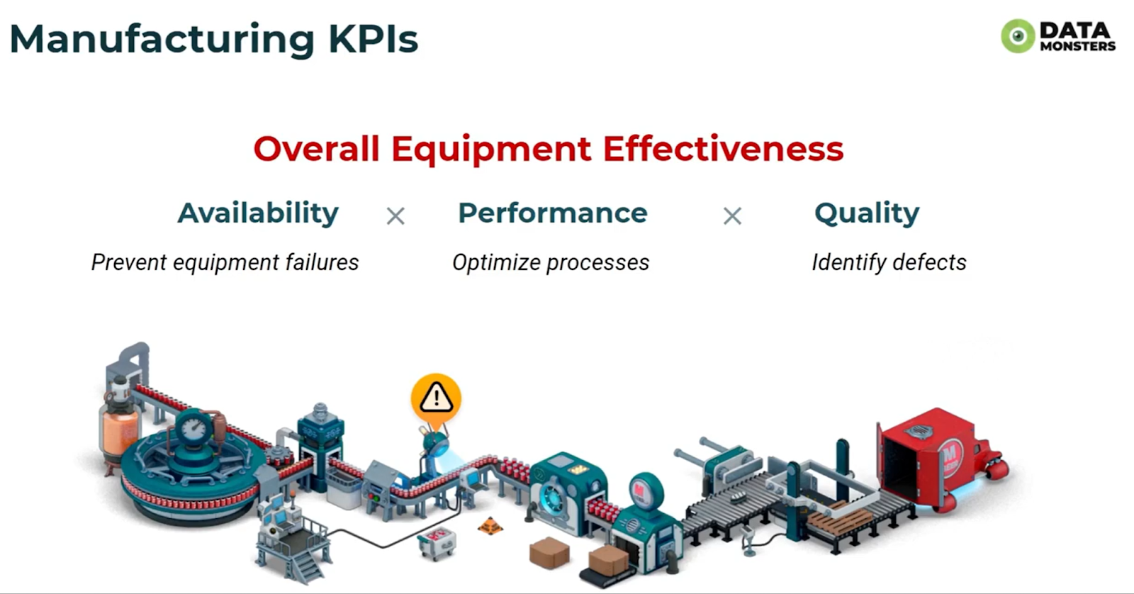
Availability is measured by the amount of uptime compared to downtime. As downtime at any part of the system can result in dramatic productivity loss, predictive maintenance is something many manufacturers are looking to in order to improve the uptime of machinery. Predictive maintenance models learn from the system and identify indicators that predict a failure. This model can alert the team prior to a failure and make recommendations about what needs to be fixed, both of which can reduce downtime.
Performance looks at how fast products are being produced compared to how fast they could be produced. With highly repetitive tasks in the manufacturing space, AI can be used to help identify the most efficient schedule based on objective function parameters, and make suggestions on where bottlenecks can be removed. Depending on the parameters, process optimization can determine the most efficient outcome based on technology variables and historical outcomes, thus maximizing throughput, minimizing cost, and reducing leftover stock.
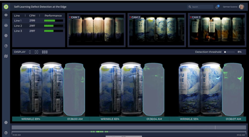
Quality of production means looking at what proportion of products are being produced without defects. Here, computer vision provides a lot of data for analysis. Manufacturers can improve the overall quality by identifying where in the process the defects are happening so they can be prevented in the future. Reducing defects and improving the overall quality of products can have a dramatic impact on not only productivity, but also revenue.
AI becomes a huge differentiator in the manufacturing space, as it reduces manual operation, and improves efficiency and the competitive position in the market with optimized costs and scheduling.
Due to the intense calculations of AI required to perform these tasks, manufacturers are bringing the compute close to sensors generating the data. Moving compute to the edge has the benefit of lowering latency and bandwidth requirements to run AI applications, ensuring the fastest and most accurate responses. With numerous compute systems on production lines, AI models are downloaded from the cloud, data is collected and processed locally. Models are fine-tuned and uploaded back to the cloud for further distribution between several edge systems.
To learn more about implementing inspections, diagnostics, and predictive maintenance in the manufacturing pipeline, check out the Data Monster’s session “Getting Started with AI in Manufacturing“.
Categories
Kubernetes for Network Engineers
 Using the same orchestration on-premise and on the public cloud allows a high level of agility and ease of operations. You can use the same API across bare metal and public clouds. Kubernetes is an open-source, container-orchestration system for automating the deployment, scaling, and management of containerized applications. It was originally designed by Google and … Continued
Using the same orchestration on-premise and on the public cloud allows a high level of agility and ease of operations. You can use the same API across bare metal and public clouds. Kubernetes is an open-source, container-orchestration system for automating the deployment, scaling, and management of containerized applications. It was originally designed by Google and is now maintained by the Cloud Native Computing Foundation.
Kubernetes is quickly becoming the new standard for deploying and managing containers in the hybrid cloud. As a network engineer, why should you care about what developers are doing with Kubernetes? Isn’t it just another application consuming network resources? Kubernetes provides a flexible and reliable platform so that developers can focus on developing and scaling their applications.
In this post, I discuss the basic building blocks of Kubernetes and some networking challenges.
Kubernetes building blocks
Kubernetes is a tool that enables you to manage cloud infrastructure and the complexities of having to manage a virtual machine or network.
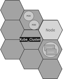
Nodes
A node is the smallest unit of computing element in Kubernetes. It is a representation of a single machine in a cluster. In most production systems, a node is usually either a physical server or a virtual machine hosted on-premises or on the cloud.
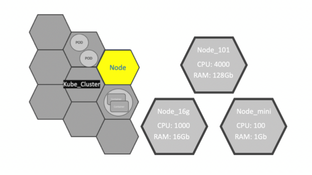
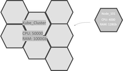
Clusters
A Kubernetes cluster is a set of node machines for running containerized applications. When you deploy applications on the cluster, the cluster intelligently handles distributing work to the individual nodes. If any nodes are added or removed, the cluster shifts workloads around as necessary. It should not matter to the application or developer which individual nodes are actually running the code.
Persistent volumes
Because applications running on the cluster are not guaranteed to run on a specific node, data cannot be saved to any arbitrary place in the file system. If an application tries to save data for later usage but is then relocated onto a new node, the data is no longer where the application expects it to be. For this reason, the traditional local storage associated with each node is treated as a temporary cache to hold applications, but any data saved locally cannot be expected to persist.
To store data permanently, Kubernetes use persistent volumes. While the CPU and RAM resources of all nodes are effectively pooled and managed by the cluster, persistent file storage is not. Instead, local or cloud stores can be attached to the cluster as a persistent volume.
Containers and microservices
Applications running on Kubernetes are packaged as Linux containers. Containers are a widely accepted standard, so there are already many prebuilt images that can be deployed on Kubernetes.
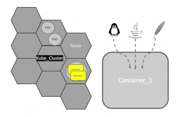
Containerization allows the creation of self-contained Linux execution environments. Any application and all its dependencies can be bundled up into a single file. Containers allow powerful continuous integration (CI) and continuous deployment (CD) pipelines to be formed, as each container can hold a specific part of an application. Containers are the underlying infrastructure for microservices.
Microservices are a software development technique, an architectural style that structures an application as a collection of loosely coupled services. The benefit of decomposing an application into different smaller services is that it improves modularity. This makes the application easier to understand, develop, test, and deploy.
Pods
Kubernetes doesn’t run containers directly. Instead, it wraps one or more containers into a higher-level structure called a Pod. Any containers in the same Pod share the same node and local network. Containers can easily communicate with other containers in the same Pod as though they were on the same machine, while maintaining a degree of isolation from others.
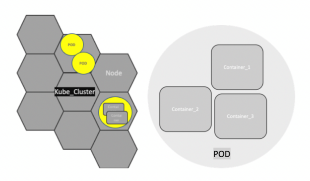
Pods are used as the unit of replication in Kubernetes. If your application becomes too heavy and a single Pod instance can’t carry the load, Kubernetes can be configured to deploy new replicas of your Pod to the cluster as necessary. Even when not under heavy load, it is standard to have multiple copies of a Pod running at any time in a production system to allow load balancing and failure resistance.
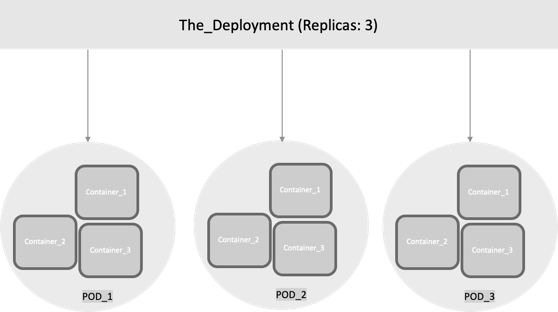
Deployments
Although Pods are the basic unit of computation in Kubernetes, they are not typically directly launched on a cluster. Instead, Pods are usually managed by one more layer of abstraction: deployment. A deployment’s purpose is to declare how many replicas of a Pod should be running at a time. When a deployment is added to the cluster, it automatically spins up the requested number of Pods, and then monitors them. If a Pod dies, the deployment automatically re-creates it.
With a deployment, you don’t have to deal with Pods manually. You can just declare the desired state of the system, and it is managed for you automatically.
Services and service meshes
A Kubernetes Service is an abstraction which defines a logical set of Pods and a policy by which to access them. Services enable loose coupling between dependent Pods.
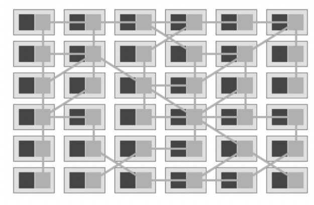
The term service mesh is used to describe the network of microservices that make up such applications and the interactions between them. As a service mesh grows in size and complexity, it can become harder to understand and manage. Its requirements can include discovery, load balancing, failure recovery, metrics, and monitoring. A service mesh also often has more complex operational requirements, like A/B testing, canary releases, rate limiting, access control, and end-to-end authentication.
One of the most popular plugins to control a service mesh is Istio, an open source, independent service, that provides the fundamentals you need to successfully run a distributed microservice architecture. Istio provides behavioral insights and operational control over the service mesh as a whole, offering a complete solution to satisfy the diverse requirements of microservice applications. With Istio, all instances of an application have their own sidecar container. This sidecar acts as a service proxy to all outgoing and incoming network traffic.
Networking
At its core, Kubernetes Networking has one important fundamental design philosophy: Every Pod has a unique IP address.
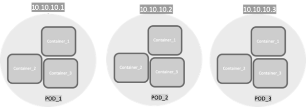
The Pod IP address is shared by all the containers inside, and it’s routable from all other Pods. A huge benefit of this IP-per-Pod model is there are no IP address or port collisions with the underlying host. There is no need to worry about what port the applications use.
With this in place, the only requirement Kubernetes has is that Pod IP addresses are routable and accessible from all the other Pods, regardless of their node.
To reduce complexity and make app porting seamless, in the Kubernetes networking model, a few rules are enforced as fundamental requirements:
- Containers can communicate with all other containers without Network Address Translation (NAT).
- Nodes can communicate with all containers without NAT and the reverse.
- The IP address that a container sees itself as is the same IP address that others see.
There are many network implementations for Kubernetes. Flannel and Calico are probably the most popular that are used as network plugins for the container network interface (CNI). CNI can be seen as the simplest possible interface between container runtimes and network implementations, with the goal of creating a generic plugin-based networking solution for containers.
Flannel can run using several encapsulation backends, with VXLAN being the recommended one. L2 connectivity is required between the Kubernetes nodes when using Flannel with VXLAN. Due to this requirement the size of the fabric might be limited, if a pure L2 network is deployed, the number of racks connected is limited to the number of ports on the spine switches.
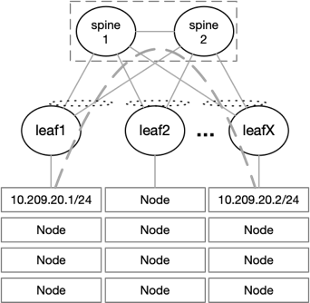
To overcome this issue, it is possible to deploy an L3 fabric with VXLAN and EVPN on the leaf level. L2 connectivity is provided to the nodes on top of a BGP-routed fabric that can scale easily. VXLAN packets coming from the nodes are encapsulated into VXLAN tunnels running between the leaf switches.
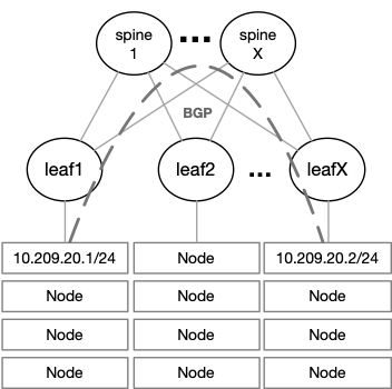
The NVIDIA Spectrum ASIC provides huge value when it comes to VXLAN throughput, latency, and scale. Most switches can support up to 128 remote VTEPs, meaning up to 128 racks in a single fabric. The NVIDIA Spectrum ASIC supports up to 750 remote VTEPs, allowing up to 750 racks in a single fabric.
NVIDIA Spectrum EVPN VXLAN differentiators
Watch the following video to learn why NVIDIA Spectrum Ethernet Switches are the best of breed platform to build a scalable, efficient, and high-performance EVPN VXLAN fabric.
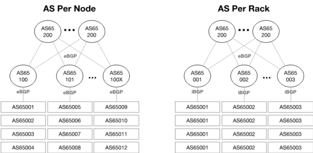
Calico AS design options
In a Calico network, each endpoint is a route. Hardware networking platforms are constrained by the number of routes they can learn. This is usually in the range of 10,000s or 100,000s of routes. Route aggregation can help, but that is usually dependent on the capabilities of the scheduler used by the orchestration software, for example, OpenStack.
When choosing a Switch for your Kubernetes deployment, make sure it has a routing table size that won’t limit your Kubernetes compute scale. The NVIDIA Spectrum ASIC provides a fully flexible table size that enables up to 176,000 IP route entries with Spectrum1 and up to 512,000 with Spectrum2, enabling the largest Kubernetes clusters run by the biggest enterprises worldwide.
Routing stack persistency across a physical network and Kubernetes
When working with Cumulus Linux OS on the switch layer, we recommend using FRR as the routing stack on your nodes, leveraging BGP unnumbered. If you are looking for a pure, open-sourced solution, consider the NVIDIA Linux Switch, which supports both FRR and BIRD as the routing stack.
Network visibility challenges with Kubernetes
Containers are automatically spun up and destroyed as needed on any server in the cluster. Because the containers are located inside a host, they can be invisible to network engineers. You might never know where they are located or when they are created and destroyed.
Operating modern agile data centers is notoriously difficult with limited network visibility and changing traffic patterns.
By using Cumulus NetQ on top of NVIDIA Spectrum switches running the Cumulus OS, you can get wide visibility into Kubernetes deployments and operate in these fast-changing, dynamic environments.
Reinforcement learning (RL) is a popular method for teaching robots to navigate and manipulate the physical world, which itself can be simplified and expressed as interactions between rigid bodies1 (i.e., solid physical objects that do not deform when a force is applied to them). In order to facilitate the collection of training data in a practical amount of time, RL usually leverages simulation, where approximations of any number of complex objects are composed of many rigid bodies connected by joints and powered by actuators. But this poses a challenge: it frequently takes millions to billions of simulation frames for an RL agent to become proficient at even simple tasks, such as walking, using tools, or assembling toy blocks.
While progress has been made to improve training efficiency by recycling simulation frames, some RL tools instead sidestep this problem by distributing the generation of simulation frames across many simulators. These distributed simulation platforms yield impressive results that train very quickly, but they must run on compute clusters with thousands of CPUs or GPUs which are inaccessible to most researchers.
In “Brax – A Differentiable Physics Engine for Large Scale Rigid Body Simulation”, we present a new physics simulation engine that matches the performance of a large compute cluster with just a single TPU or GPU. The engine is designed to both efficiently run thousands of parallel physics simulations alongside a machine learning (ML) algorithm on a single accelerator and scale millions of simulations seamlessly across pods of interconnected accelerators. We’ve open sourced the engine along with reference RL algorithms and simulation environments that are all accessible via Colab. Using this new platform, we demonstrate 100-1000x faster training compared to a traditional workstation setup.
 |
| Three typical RL workflows. The left shows a typical workstation flow: on a single machine, with the environment on CPU, training takes hours or days. The middle shows a typical distributed simulation flow: training takes minutes by farming simulation out to thousands of machines. The right shows the Brax flow: learning and large batch simulation occur side by side on a single CPU/GPU chip. |
Physics Simulation Engine Design Opportunities
Rigid body physics are used in video games, robotics, molecular dynamics, biomechanics, graphics and animation, and other domains. In order to accurately model such systems, simulators integrate forces from gravity, motor actuation, joint constraints, object collisions, and others to simulate the motion of a physical system across time.
 |
| Simulation of three spherical bodies, a wall, two joints, and one actuator. For each simulation timestep, forces and torques are integrated together to update the positions, rotations, and velocities of each physical body. |
Taking a closer look at how most physics simulation engines are designed today, there are a few large opportunities to improve efficiency. As we noted above, a typical robotics learning pipeline places a single learner in a tight feedback with many simulations in parallel, but upon analyzing this architecture, one finds that:
- This layout imposes an enormous latency bottleneck. Because the data must travel over the network within a datacenter, the learner must wait for 10,000+ nanoseconds to fetch experience from the simulator. Were this experience instead already on the same device as the learner’s neural network, latency would drop to <1 nanosecond.
- The computation necessary for training the agent (one simulation step, followed by one update of the agent’s neural network) is overshadowed by the computation spent packaging the data (i.e., marshalling data within the engine, then into a wire format such as protobuf, then into TCP buffers, and then undoing all these steps on the learner side).
- The computations happening within each simulator are remarkably similar, but not exactly the same.
Brax Design
In response to these observations, Brax is designed so that its physics calculations are exactly the same across each of its thousands of parallel environments by ensuring that the simulation is free of branches (i.e., simulation “if” logic that diverges as a result of the environment state). An example of a branch in a physics engine is the application of a contact force between a ball and a wall: different code paths will execute depending on whether the ball is touching the wall. That is, if the ball contacts the wall, separate code for simulating the ball’s bounce off the wall will execute. Brax employs a mix of the following three strategies to avoid branching:
- Replace the discrete branching logic with a continuous function, such as approximating the ball-wall contact force using a signed distance function. This approach results in the most efficiency gains.
- Evaluate the branch during JAX’s just-in-time compile. Many branches based on static properties of the environment, such as whether it’s even possible for two objects to collide, may be evaluated prior to simulation time.
- Run both sides of the branch during simulation but then select only the required results. Because this executes some code that isn’t ultimately used, it wastes operations compared to the above.
Once the calculations are guaranteed to be exactly uniform, the entire training architecture can be reduced in complexity to be executed on a single TPU or GPU. Doing so removes the computational overhead and latency of cross-machine communication. In practice, these changes lower the cost of training by 100x-1000x for comparable workloads.
Brax Environments
Environments are tiny packaged worlds that define a task for an RL agent to learn. Environments contain not only the means to simulate a world, but also functions, such as how to observe the world and the definition of the goal in that world.
A few standard benchmark environments have emerged in recent years for testing new RL algorithms and for evaluating the impact of those algorithms using metrics commonly understood by research scientists. Brax includes four such ready-to-use environments that come from the popular OpenAI gym: Ant, HalfCheetah, Humanoid, and Reacher.
 |
 |
 |
 |
| From left to right: Ant, HalfCheetah, Humanoid, and Reacher are popular baseline environments for RL research. |
Brax also includes three novel environments: dexterous manipulation of an object (a popular challenge in robotics), generalized locomotion (an agent that goes to a target placed anywhere around it), and a simulation of an industrial robot arm.
 |
 |
 |
| Left: Grasp, a claw hand that learns dexterous manipulation. Middle: Fetch, a toy, box-like dog learns a general goal-based locomotion policy. Right: Simulation of UR5e, an industrial robot arm. |
Performance Benchmarks
The first step for analyzing Brax’s performance is to measure the speed at which it can simulate large batches of environments, because this is the critical bottleneck to overcome in order for the learner to consume enough experience to learn quickly.
These two graphs below show how many physics steps (updates to the state of the environment) Brax can produce as it is tasked with simulating more and more environments in parallel. The graph on the left shows that Brax scales the number of steps per second linearly with the number of parallel environments, only hitting memory bandwidth bottlenecks at 10,000 environments, which is not only enough for training single agents, but also suitable for training entire populations of agents. The graph on the right shows two things: first, that Brax performs well not only on TPU, but also on high-end GPUs (see the V100 and P100 curves), and second, that by leveraging JAX’s device parallelism primitives, Brax scales seamlessly across multiple devices, reaching hundreds of millions of physics steps per second (see the TPUv3 8×8 curve, which is 64 TPUv3 chips directly connected to each other over a high speed interconnect) .
 |
| Left: Scaling of the simulation steps per second for each Brax environment on a 4×2 TPU v3. Right: Scaling of the simulation steps per second for several accelerators on the Ant environment. |
Another way to analyze Brax’s performance is to measure its impact on the time it takes to run a reinforcement learning experiment on a single workstation. Here we compare Brax training the popular Ant benchmark environment to its OpenAI counterpart, powered by the MuJoCo physics engine.
In the graph below, the blue line represents a standard workstation setup, where a learner runs on the GPU and the simulator runs on the CPU. We see that the time it takes to train an ant to run with reasonable proficiency (a score of 4000 on the y axis) drops from about 3 hours for the blue line, to about 10 seconds using Brax on accelerator hardware. It’s interesting to note that even on CPU alone (the grey line), Brax performs more than an order of magnitude faster, benefitting from learner and simulator both sitting in the same process.
 |
| Brax’s optimized PPO versus a standard GPU-backed PPO learning the MuJoCo-Ant-v2 environment, evaluated for 10 million steps. Note the x-axis is log-wallclock-time in seconds. Shaded region indicates lowest and highest performing seeds over 5 replicas, and solid line indicates mean. |
Physics Fidelity
Designing a simulator that matches the behavior of the real world is a known hard problem that this work does not address. Nevertheless, it is useful to compare Brax to a reference simulator to ensure it is producing output that is at least as valid. In this case, we again compare Brax to MuJoCo, which is well-regarded for its simulation quality. We expect to see that, all else being equal, a policy has a similar reward trajectory whether trained in MuJoCo or Brax.
 |
| MuJoCo-Ant-v2 vs. Brax Ant, showing the number of environment steps plotted against the average episode score achieved for the environment. Both environments were trained with the same standard implementation of SAC. Shaded region indicates lowest and highest performing seeds over five runs, and solid line indicates the mean. |
These curves show that as the reward rises at about the same rate for both simulators, both engines compute physics with a comparable level of complexity or difficulty to solve. And as both curves top out at about the same reward, we have confidence that the same general physical limits apply to agents operating to the best of their ability in either simulation.
We can also measure Brax’s ability to conserve linear momentum, angular momentum, and energy.
 |
| Linear momentum (left), angular momentum (middle), and energy (right) non-conservation scaling for Brax as well as several other physics engines. The y-axis indicates drift from the expected calculation (higher is smaller drift, which is better), and the x axis indicates the amount of time being simulated. |
This measure of physics simulation quality was first proposed by the authors of MuJoCo as a way to understand how the simulation drifts off course as it is tasked with computing larger and larger time steps. Here, Brax performs similarly as its neighbors.
Conclusion
We invite researchers to perform a more qualitative measure of Brax’s physics fidelity by training their own policies in the Brax Training Colab. The learned trajectories are recognizably similar to those seen in OpenAI Gym.
Our work makes fast, scalable RL and robotics research much more accessible — what was formerly only possible via large compute clusters can now be run on workstations, or for free via hosted Google Colaboratory. Our Github repository includes not only the Brax simulation engine, but also a host of reference RL algorithms for fast training. We can’t wait to see what kind of new research Brax enables.
Acknowledgements
We’d like to thank our paper co-authors: Anton Raichuk, Sertan Girgin, Igor Mordatch, and Olivier Bachem. We also thank Erwin Coumans for advice on building physics engines, Blake Hechtman and James Bradbury for providing optimization help with JAX and XLA, and Luke Metz and Shane Gu for their advice. We’d also like to thank Vijay Sundaram, Wright Bagwell, Matt Leffler, Gavin Dodd, Brad Mckee, and Logan Olson, for helping to incubate this project.
1 Due to the complexity of the real world, there is also ongoing research exploring the physics of deformable bodies. ↩
 Workshops are conducted live in a virtual classroom environment with expert guidance from NVIDIA-certified instructors.
The NVIDIA Deep Learning Institute (DLI) extended its popular public workshop summer series through September 2021. These workshops are conducted live in a virtual classroom environment with expert guidance from NVIDIA-certified instructors. Participants have access to fully configured GPU-accelerated servers in the cloud to perform hands-on exercises.
To register, visit our website. Space is limited so we encourage you to sign up early.
Here is our current public workshop schedule:
August
Fundamentals of Deep Learning
Wed, August 25, 9:00 a.m. to 5:00 p.m. PDT (NALA)
Fundamentals of Accelerated Computing with CUDA Python
Thu, August 26, 9:00 a.m. to 5:00 p.m. CEST (EMEA)
September
Fundamentals of Deep Learning
Thu, September 16, 9:00 a.m. to 5:00 p.m. CEST (EMEA)
Deep Learning for Industrial Inspection
Tue, September 21, 9:00 a.m. to 5:00 p.m. CEST (EMEA)
Tue, September 21, 9:00 a.m. to 5:00 p.m. PDT (NALA)
Applications of AI for Anomaly Detection
Wed, September 22, 9:00 a.m. to 5:00 p.m. CEST (EMEA)
Wed, September 22, 9:00 a.m. to 5:00 p.m. PDT (NALA)
Building Transformer-Based Natural Language Processing Applications
Thu, September 23, 9:00 a.m. to 5:00 p.m. PDT (NALA)
Visit the DLI website for details on each course and the full schedule of upcoming instructor-led workshops, which is regularly updated with new training opportunities.
For more information, e-mail nvdli@nvidia.com.
Every teacher has a story about the moment a light switched on for one of their students. David Tseng recalls a high school senior in Taipei excited at a summer camp to see a robot respond instantly when she updated her software. After class, she had a lot of questions and later built an AI-powered Read article >
The post A Sparkle in Their AIs: Students Worldwide Rev Robots with Jetson Nano appeared first on The Official NVIDIA Blog.
 Edge computing has been around for a long time, but has recently become a hot topic because of the convergence of three major trends – IoT, 5G, and AI.
Edge computing has been around for a long time, but has recently become a hot topic because of the convergence of three major trends – IoT, 5G, and AI.
IoT devices are becoming smarter and more capable, increasing the breadth of applications that can be deployed on them and the environments they can be deployed in. Simultaneously, recent advancements in 5G capabilities give confidence that this technology will soon be able to connect IoT devices wirelessly anywhere they are deployed. In fact, analysts predict that there will be over 1 billion 5G connected devices by 2023. Lastly, AI successfully moved from research projects into practical applications, changing the landscape for retailers, factories, hospitals, and many more.
So what does the convergence of these trends mean? An explosion in the number of IoT devices deployed.
Experts estimate there are over 30 billion IoT devices installed today, and Arm predicts that by 2035, there will be over 1 trillion devices. With that many IoT devices deployed, the amount of data collected skyrocketed, putting strain on current cloud infrastructures. Organizations soon found themselves in a position where the AI applications they deployed needed large amounts of data to generate compelling insights, but the latency for their cloud infrastructure to process data and send insights back to the edge were unsustainable. So they turned to edge computing.
By putting the processing power at the location that sensors are collecting data, organizations reduce the latency for applications to deliver insights. For some situations, such as autonomous machines at factories, the latency reduction represents a critical safety component.
That is where NVIDIA comes in. The NVIDIA Edge AI solution offers a complete end-to-end AI platform for deploying AI at the edge. It starts with NVIDIA-Certified Systems.
NVIDIA-Certified Systems combine the computing power of NVIDIA GPUs with secure high-bandwidth, low-latency networking solutions from NVIDIA. Validated for performance, functionality, scalability, and security – IT teams ensure AI workloads deployed from the NGC catalog, NVIDIA’s GPU-optimized hub of HPC and AI software, run at full performance. These servers are backed by enterprise-grade support, including direct access to NVIDIA experts, minimizing system downtime and maximizing user productivity.
To build and accelerate applications running on NVIDIA-Certified Systems, NVIDIA offers an extensive toolkit of SDKs, application frameworks, and other tools designed to help developers build AI applications for every industry. These include pretrained models, training scripts, optimized framework containers, inference engines, and more. With these tools, organizations get a head start on building unique AI applications regardless of workload or industry.
Once organizations have the hardware to accelerate AI and an AI application to deploy, the next step is to ensure that there is infrastructure in place to manage and scale the application. Without a platform to manage AI at the edge, organizations face the difficult and costly task of manually updating systems at edge locations every time a new software update is released.
NVIDIA Fleet Command is a cloud service that securely deploys, manages, and scales AI applications across distributed edge infrastructure. Purpose-built for AI, Fleet Command is a turnkey solution for AI lifecycle management, offering streamlined deployments, layered security, and detailed monitoring capabilities — so organizations can go from zero to AI in minutes.
The complete edge AI solution gives organizations the tools needed to build an end-to-end edge deployment. KION Group, the number one global supply chain solutions provider, uses NVIDIA solutions to fulfill order faster and more efficiently.
To learn more about NVIDIA edge AI solutions, check out Deploying and Accelerating AI at the Edge With the NVIDIA EGX Platform.