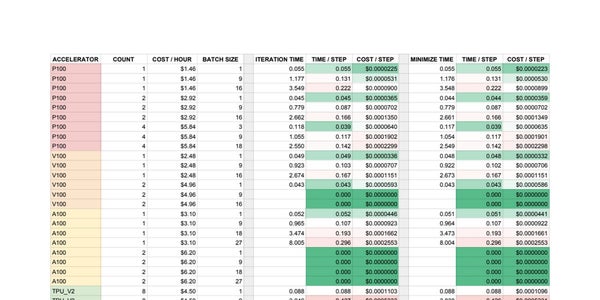
I’m currently doing some tests in preparation for my first real bit of training. I’m using Google Cloud AI Platform to train, and am trying to find the optimal machine setup. It’s a work in progress, but here’s a table I’m putting together to get a sense of the efficiency of each setup. On the left you’ll see the accelerator type, ordered from least to most expensive. Here you’ll also find the number of accelerator’s used, the cost per hour, and the batch size. To the right are the average time it took to complete an entire training iteration and how long it took to complete the minimization step. You’ll notice that the values are almost identical for each setup; I’m using Google Research’s SEED RL, so I thought to record both values since I’m not sure exactly everything that happens between iterations. Turns out it’s not much. There’s also a calculation of the the time it takes to complete a single “step” (aka, a single observation from a single environment), as well as the average cost per step.
So, the problem. I was under the assumption that batching with a GPU or TPU would increase the efficiency of the training. Instead, it turns out that a batch size of 1 is the most efficient both in time per step and cost per step. I’m still fairly new to ML so maybe it’s just a matter of me being uninformed, but this goes against everything I thought I knew about ML training. Since I’m using Google’s own SEED codebase I would assume that it’s not a problem with the code, but I can’t be sure about that.
Is this just a matter of me misunderstanding how training works, or am I right in thinking something is really off?
NVIDIA Optical Flow SDK exposes the APIs to use this Optical Flow hardware (also referred to as NVOFA) to accelerate applications.
The NVIDIA Turing architecture introduced a new hardware functionality for computing optical flow between a pair of images with very high performance. NVIDIA Optical Flow SDK exposes the APIs to use this Optical Flow hardware (also referred to as NVOFA) to accelerate applications. We are excited to announce the availability of Optical Flow SDK 3.0 with the following new features:
DirectX 12 Optical Flow API
Forward-Backward Optical Flow via a single API
Global Flow vector
DirectX 12 Optical Flow API
DirectX 12 is a low-level programming API from Microsoft which reduces driver overhead in comparison to its predecessor DirectX 11. DirectX 12 provides more flexibility and fine-grained control to the developer. Developers can now take advantage of the low-level programming APIs in DirectX 12 and optimize their applications to give better performance over earlier DirectX versions – at the same time, the client application, on its own, must take care of resource management, synchronization, etc. DirectX 12 has rapidly grown amongst game titles and other graphics applications.
Optical Flow SDK 3.0 enables DirectX 12 applications to use the NVIDIA Optical Flow engine. The computed optical flow can be used to increase frame rate in games and videos for smoother experience or in object tracking. To increase the frame rate, Frame Rate Up Conversion (FRUC) techniques are used by inserting interpolated frames between original frames. Interpolation algorithms use the flow between frame pair(s) to generate the intermediate frame.
All generations of Optical Flow Hardware support DirectX 12 Optical Flow interface. The Optical Flow SDK package contains header(s), sample applications that demonstrate the usage, C++ wrapper classes which can be re-used or modified as required and documentation. All the other components for accessing the Optical Flow hardware are included in the NVIDIA display driver. DirectX 12 Optical Flow API is supported on Windows 20H1 or later operating system.
Barring the explicit synchronization, DirectX 12 Optical Flow API is designed to be close to the other interfaces that are already available in the SDK (CUDA and DirectX 11). The DirectX 12 Optical Flow API consists of three core functions: initialization, flow estimation and destruction.
Initialization and destroy APIs are same across all interfaces but Execute API differs between DirectX 12 and other interfaces i.e., DirectX 11 and CUDA. Even though most of the parameters passed to the Execute API in DirectX 12 are same as those in other two interfaces, there are some functional differences. Synchronization in DirectX 11 and CUDA interfaces is automatically taken care by OS runtime and driver. However, in DirectX 12, additional information about fence and fence values are required as input parameters to the Execute API. These fence objects will be used to synchronize the CPUGPU and GPUGPU operations. For more details, please refer to the programming guide included with the Optical Flow SDK.
Buffer management API interface in DirectX 12 also needs fence objects for synchronization.
The Optical Flow output quality is same across all interfaces. Performance in DirectX 12 should be very close compared to the other two interfaces.
Forward-Backward Optical Flow (FB flow)
No Optical Flow algorithm can give 100% accurate flow. The flow is typically distorted in occluded regions. Sometimes, the cost provided by the NVOFA may not also represent true confidence of the flow. One simple check usually employed is to compare the forward and backward flow. If the Euclidean distance between forward flow and backward flow exceeds a threshold, the flow can be marked as invalid.
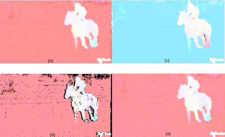
To estimate flow in both directions, client must call the Execute API twice: one call with input and reference images and second call after reversing the input and reference images. Calling the Optical Flow Execute API two times like this can result in suboptimal performance due to overheads such as context switching, thread switching etc. Optical Flow SDK 3.0 exposes a new API to generate flow in both directions in a single Execute call. This feature can be enabled by setting NV_OF_INIT_PARAMS::predDirection to NV_OF_PRED_DIRECTION_BOTH in initialization and providing necessary buffers to receive backward flow and/or cost in NV_OF_EXECUTE_OUTPUT_PARAMS/NV_OF_EXECUTE_OUTPUT_PARAMS_D3D12::bwdOutputBuffer, NV_OF_EXECUTE_OUTPUT_PARAMS/NV_OF_EXECUTE_OUTPUT_PARAMS_D3D12::bwdOutputCostBuffer.
Figure 2. (b) Forward Flow, (c) Backward Flow, (d) Consistency Check. Black pixels in the image shows inconsistent flow, (e) Nearest Neighbor Infill
Once the flow is generated in both directions, client application can compare the flow vectors of both directions, discard the inaccurate ones based on a suitable criteria (e.g. Euclidian distance between forward and backward flow vectors), and use hole filling algorithms to fill such discarded flow vectors.
Note that the output quality of FB flow could be different from unidirectional flow due to some optimizations.
Sample code that demonstrates FB flow API programming and consistency check:
Global flow in a video sequence or game is caused by camera panning motion. Global flow estimation is an important tool widely used in image segmentation, video stitching or motion-based video analysis applications.
Global Flow vector can also be heuristically used in calculating background motion. Once background motion is estimated, this can be used to fill the flow vectors in occluded regions. It can also be used to handle collisions of warped pixels in interpolated frames.
Global flow is calculated on the forward flow vectors, based on frequency of the occurrence and a few other heuristics.
To enable generation of global flow, initialization API needs to set the flag NV_OF_INIT_PARAMS:: enableGlobalFlow and provide the additional buffer NV_OF_EXECUTE_OUTPUT_PARAMS/NV_OF_EXECUTE_OUTPUT_PARAMS_D3D12::globalFlowBuffer in Execute API.
Hosted by the Department of Veterans Affairs (VA), the sprint is designed to foster collaboration with industry and academic partners on AI-enabled tools that leverage federal data to address a need for veterans.
Five NVIDIA Inception partners were named finalists at the 2020-2021 Artificial Intelligence Tech Sprint, a competition aimed at improving healthcare for veterans using the latest AI technology. Hosted by the Department of Veterans Affairs (VA), the sprint is designed to foster collaboration with industry and academic partners on AI-enabled tools that leverage federal data to address a need for veterans. See the official news release for more details about the competition.
Participating teams gave presentations and demonstrations judged by panels of Veterans and other experts. 44 teams from industry and universities participated, addressing a range of health care challenges such as chronic conditions management, cancer screening, rehabilitation, patient experiences and more.
Majority of the solutions from NVIDIA Inception partners were powered by NVIDIA Clara Guardian, a smart hospital solution for patient monitoring, mental health, and patient care.
JumpStartCSR created ‘Holmz’ – a data source agnostic explainable AI (XAI) that provides a digital physical therapy to prevent and treat overexertion/repetitive stress injuries. Holmz can predict plantar fasciitis and identify root causes two weeks in advance of its occurrence with 97% accuracy and 99% accuracy one week in advance of occurrence. Holmz is also capable of predicting fatigue related falls and identifying their root causes 15 minutes in advance of their occurrence with 99% accuracy. The trained solutions are 4 to 5x faster using TensorFlow with NVIDIA T4 GPUs on AWS. They are piloting their XAI with the VA’s Physical Medicine and Rehabilitation group and expanding their digital physical therapy solution to include performance improvement and prediction for the US Army.
Ouva is an Autonomous Remote Monitoring and Ambient Intelligence platform that is designed to improve patient safety and operational efficiency. Their solution leverages cuDNN, TensorRT, Transfer Learning Toolkit in NVIDIA Clara Guardian and runs on an NVIDIA RTX 6000 GPU. During the course of VA tech sprint, Ouva was able to predict sepsis infection 24 hours ahead of clinical diagnosis by looking at nine biomarkers from EMR collected from 40,000 patients. By processing data from telehealth cameras with AI, Ouva allows nurses to keep an eye on more patients at remote or isolation conditions. They have started deploying their remote care monitoring solution in Europe and piloting it in the US. Their near-term goal is to combine Ouva’s unique patient activity data with Electronic Medical Records (EMR) to uniquely predict more cases like Sepsis with increased accuracy.
PATH Decision Support Software, a GPU-accelerated expert system that recommends drug regimens for patients with type 2 diabetes. Their solution was developed on CUDA using NVIDIA GPUs on AWS and achieved 20x speedup. The software’s recommendations have shown a 2.1-point reduction in HbA1c and a $770/patient/year reduction in unplanned diabetes-related Medicaid claims. The team is currently working on EMR integration and expanding the list of medicines it can evaluate.
Dialisa is a digital nutritional Intervention platform that detects onset and monitors progression of chronic kidney disease (CKD) and delivers digital nutritional intervention to delay the progress of the disease. They use TensorFlow and CUDA optimized on NVIDIA GPUs on AWS, achieving an accuracy of 93.2% in detecting onset of CKD using generic longitudinal dataset provided by the National Artificial Intelligence Institute (NAII) at the Veterans Administrations. Dialisa looks to demonstrate the feasibility of their algorithms and remote monitoring platform in the veterans community, and welcome additional clinical partners to conduct pilot study in the general population.
KELLS, an AI-powered dental diagnostic platform, used TensorFlow and PyTorch optimized on NVIDIA T4 GPUs on AWS P3 instances and achieved 3x higher efficiency in training than previously used AWS G4 instances. KELLS’ technology has demonstrated to improve accuracy of detecting common dental pathologies up to 30% for average dentists, especially for detecting early signs of oral disease, enabling more timely and effective preventative care. They continue to expand their platform to support more clinical findings across different data modalities and increase quality and accessibility of dental care for patients.
“We were overwhelmed with the overall quality of proposals in this very competitive cycle, it’s a great tribute to our mission to serve our veterans,” said Artificial Intelligence Tech Sprint lead Rafael Fricks. “Very sophisticated AI capabilities are more accessible than ever; a few years ago these proposals wouldn’t have been possible outside the realm of very specialized high performance computing.”
NVIDIA looks forward to providing continued support to these winning Inception Partners in the coming Pilot Implementation program phase, and to the contributions their AI solutions will make to the important VA/VHA healthcare mission serving our Nation’s veterans.
Targeting areas populated with disease-carrying mosquitoes just got easier thanks to a new study. The research, recently published in IEEE Explore, uses deep learning to recognize tiger mosquitoes from images taken by citizen scientists with near perfect accuracy. “Identifying the mosquitoes is fundamental, as the diseases they transmit continue to be a major public health … Continued
Targeting areas populated with disease-carrying mosquitoes just got easier thanks to a new study. The research, recently published in IEEE Explore, uses deep learning to recognize tiger mosquitoes from images taken by citizen scientists with near perfect accuracy.
“Identifying the mosquitoes is fundamental, as the diseases they transmit continue to be a major public health issue,” said lead author Gereziher Adhane.
The study, from researchers at the Scene understanding and artificial intelligence (SUNAI) research group, of the Universitat Oberta de Catalunya’s (UOC) Faculty of Computer Science, Multimedia and Telecommunications and of the eHealth Center, uses images from the Mosquito Alert app. Developed in Spain and currently expanding globally, the platform brings together citizens, entomologists, public health authorities, and mosquito control services to reduce mosquito-borne diseases.
Anyone in the world can upload geo-tagged images of mosquitoes to the app. Once submitted, three expert entomologists inspect and validate the images before they are added to the database, classified, and mapped.
Travel and migration, along with climate change and urbanization has broadened the range and habitat of mosquitoes. Quick identification of species such as the tiger mosquito – known to transmit dengue, Zika, chikungunya, and yellow fever – remains a key step in assisting relevant authorities to curb their spread.
Sample of tiger [first row] and non-tiger [second row] mosquitoes from the Mosquito Alert data set. Credit: G. Adhane et al/IEEE Explore
“This type of analysis depends largely on human expertise and requires the collaboration of professionals, is typically time-consuming, and is not cost-effective because of the possible rapid propagation of invasive species,” said Adhane. “This is where neural networks can play a role as a practical solution for controlling the spread of mosquitoes.”
The research team developed a deep convolutional neural network (CNN) that distinguishes between mosquito species. Starting with a pre-trained model, they fine-tuned it using the hand-labeled Mosquito Alert dataset. Using NVIDIA GPUs and the cuDNN-accelerated PyTorch deep learning framework, the classification models were taught to pinpoint tiger mosquitoes based on identifiable morphological features such as white stripes on the legs, abdominal patches, head, and thorax shape.
Deep learning models typically rely on millions of samples. However, using only 6,378 images of both tiger and non-tiger mosquitoes from Mosquito Alert, the researchers were able to train the model with about 94% accuracy.
“The neural network we have developed can perform as well or nearly as well as a human expert and the algorithm is sufficiently powerful to process massive amounts of images,” said Adhane.
According to the researchers, as Mosquito Alert scales up, the study can be expanded to classify multiple species of mosquitoes and their breeding sites across the globe.
“The model we have developed could be used in practical applications with small modifications to work with mobile apps. Using this trained network it is possible to make predictions about images of mosquitoes taken using smartphones efficiently and in real time,” Adhane said.
I’m kind of a noob at tensorflow, built a few classifieds but that’s it. I’m now trying to use the tensorflow object detection API, but the command to install the dependencies takes hours to install everything.
This would be fine if it weren’t for the fact that I’m in a research setting that requires me to run in a docker container. I could create a custom docker image and solve it that way, but does anyone know how to make this process go faster?
Posted by Pablo Samuel Castro, Staff Software Engineer, Google Research
It is widely accepted that the enormous growth of deep reinforcement learning research, which combines traditional reinforcement learning with deep neural networks, began with the publication of the seminal DQN algorithm. This paper demonstrated the potential of this combination, showing that it could produce agents that could play a number of Atari 2600 games very effectively. Since then, there have been severalapproaches that have built on and improved the original DQN. The popular Rainbow algorithm combined a number of these recent advances to achieve state-of-the-art performance on the ALE benchmark. This advance, however, came at a very high computational cost, which has the unfortunate side effect of widening the gap between those with ample access to computational resources and those without.
In “Revisiting Rainbow: Promoting more Insightful and Inclusive Deep Reinforcement Learning Research”, to be presented at ICML 2021, we revisit this algorithm on a set of small- and medium-sized tasks. We first discuss the computational cost associated with the Rainbow algorithm. We explore how the same conclusions regarding the benefits of combining the various algorithmic components can be reached with smaller-scale experiments, and further generalize that idea to how research done on a smaller computational budget can provide valuable scientific insights.
The Cost of Rainbow A major reason for the computational cost of Rainbow is that the standards in academic publishing often require evaluating new algorithms on large benchmarks like ALE, which consists of 57 Atari 2600 games that reinforcement learning agents may learn to play. For a typical game, it takes roughly five days to train a model using a Tesla P100 GPU. Furthermore, if one wants to establish meaningful confidence bounds, it is common to perform at least five independent runs. Thus, to train Rainbow on the full suite of 57 games required around 34,200 GPU hours (or 1425 days) in order to provide convincing empirical performance statistics. In other words, such experiments are only feasible if one is able to train on multiple GPUs in parallel, which can be prohibitive for smaller research groups.
We evaluate on a set of four classic control environments, which can be fully trained in 10-20 minutes (compared to five days for ALE games):
Upper left: In CartPole, the task is to balance a pole on a cart that the agent can move left and right. Upper right: In Acrobot, there are two arms and two joints, where the agent applies force to the joint between the two arms in order to raise the lower arm above a threshold. Lower left: In LunarLander, the agent is meant to land the spaceship between the two flags. Lower right: In MountainCar, the agent must build up momentum between two hills to drive to the top of the rightmost hill.
We investigated the effect of both independently adding each of the components to DQN, as well as removing each from the full Rainbow algorithm. As in the original Rainbow paper, we find that, in aggregate, the addition of each of these algorithms does improve learning over the base DQN. However, we also found some important differences, such as the fact that distributional RL — commonly thought to be a positive addition on its own — does not always yield improvements on its own. Indeed, in contrast to the ALE results in the Rainbow paper, in the classic control environments, distributional RL only yields an improvement when combined with another component.
Each plot shows the training progress when adding the various components to DQN. The x-axis is training steps,the y-axis is performance (higher is better).
Each plot shows the training progress when removing the various components from Rainbow. The x-axis is training steps,the y-axis is performance (higher is better).
We also re-ran the Rainbow experiments on the MinAtar environment, which consists of a set of five miniaturized Atari games, and found qualitatively similar results. The MinAtar games are roughly 10 times faster to train than the regular Atari 2600 games on which the original Rainbow algorithm was evaluated, but still share some interesting aspects, such as game dynamics and having pixel-based inputs to the agent. As such, they provide a challenging mid-level environment, in between the classic control and the full Atari 2600 games.
When viewed in aggregate, we find our results to be consistent with those of the original Rainbow paper — the impact resulting from each algorithmic component can vary from environment to environment. If we were to suggest a single agent that balances the tradeoffs of the different algorithmic components, our version of Rainbow would likely be consistent with the original, in that combining all components produces a better overall agent. However, there are important details in the variations of the different algorithmic components that merit a more thorough investigation.
Beyond the Rainbow When DQN was introduced, it made use of the Huber loss and the RMSProp Optimizer. It has been common practice for researchers to use these same choices when building on DQN, as most of their effort is spent on other algorithmic design decisions. In the spirit of reassessing these assumptions, we revisited the loss function and optimizer used by DQN on a lower-cost, small-scale classic control and MinAtar environments. We ran some initial experiments using the Adam optimizer, which has lately been the most popular optimizer choice, combined with a simpler loss function, the mean-squared error loss (MSE). Since the selection of optimizer and loss function is often overlooked when developing a new algorithm, we were surprised to see that we observed a dramatic improvement on all the classic control and MinAtar environments.
We thus decided to evaluate the different ways of combining the two optimizers (RMSProp and Adam) with the two losses (Huber and MSE) on the full ALE suite (60 Atari 2600 games). We found that Adam+MSE is a superior combination than RMSProp+Huber.
Measuring the improvement Adam+MSE gives over the default DQN settings (RMSProp + Huber); higher is better.
Additionally, when comparing the various optimizer-loss combinations, we find that when using RMSProp, the Huber loss tends to perform better than MSE (illustrated by the gap between the solid and dotted orange lines).
Normalized scores aggregated over all 60 Atari 2600 games, comparing the different optimizer-loss combinations.
Conclusion On a limited computational budget we were able to reproduce, at a high-level, the findings of the Rainbow paper and uncover new and interesting phenomena. Evidently it is much easier to revisit something than to discover it in the first place. Our intent with this work, however, was to argue for the relevance and significance of empirical research on small- and medium-scale environments. We believe that these less computationally intensive environments lend themselves well to a more critical and thorough analysis of the performance, behaviors, and intricacies of new algorithms.
We are by no means calling for less emphasis to be placed on large-scale benchmarks. We are simply urging researchers to consider smaller-scale environments as a valuable tool in their investigations, and reviewers to avoid dismissing empirical work that focuses on smaller-scale environments. By doing so, in addition to reducing the environmental impact of our experiments, we will get both a clearer picture of the research landscape and reduce the barriers for researchers from diverse and often underresourced communities, which can only help make our community and scientific advances stronger.
Acknowledgments Thank you to Johan, the first author of this paper, for his hard work and persistence in seeing this through! We would also like to thank Marlos C. Machado, Sara Hooker, Matthieu Geist, Nino Vieillard, Hado van Hasselt, Eleni Triantafillou, and Brian Tanner for their insightful comments on this work.
Developers can use the new viisights wise application powered by GPU-accelerated AI technologies to help organizations and municipalities worldwide avoid operational hazards and risk in their most valuable spaces.
Developers can use the new viisights wise application powered by GPU-accelerated AI technologies to help organizations and municipalities worldwide avoid operational hazards and risk in their most valuable spaces.
With conventional imaging and analytics solutions, AI vision is used to detect the presence of people and objects and their basic attributes to better understand how a physical space is being used. For example, is there a pedestrian, cyclist, or vehicle on a roadway? While understanding what’s happening on a road or in a retail store is important, predicting what might happen next is critical to taking this vision to the next level and building even smarter spaces.
viisights — an NVIDIA Metropolis partner — helps cities and enterprises make better decisions faster by offering an AI-enabled platform that analyzes complex behavior within video content. viisights uses the NVIDIA Deepstream SDK to accelerate their development workflow for its video analytics pipeline, cutting development time by half. DeepStream is a path to developing highly optimized video analysis pipelines including video decoding, multi-stream processing and accelerated image transformations in real-time, critical for high performance video analytics applications. For deployment, viisights uses NVIDIA TensorRT to further accelerate their application’s inference throughput at the edge with INT8 calibration.
The viisights Wise application recognizes and classifies over 200 different types of objects and dozens of different types of actions and events. The ability to recognize that a person is running, falling, or throwing an object provides a far richer and more holistic understanding of how spaces are being used. By using viisights Wise, operations teams can gain deeper insights and identify behavioral patterns that can predict what might happen next. viisights Wise can process over 20 video streams on a single GPU in near real-time.
viisights technology protects public privacy, as it only analyzes general behavior patterns of individuals and groups and does not identify specifics like faces or license plates. Because the application only analyzes behavior patterns, viisights technology is incredibly easy to use, further increasing ROI.
Real-world situations and use cases for viisights Wise include:
Hazard Detection: Detect operational hazards in real-time. These include large objects that might block human or vehicle mobility in both outdoor and indoor surroundings such as streets, sidewalks, production floors, and operational areas in transportation hubs. It can even detect environmental hazards like smoke or fire in outdoor areas where smoke detectors cannot be installed.
Traffic Management: Cities can make informed decisions on how to best modify roadways, traffic patterns, public transit infrastructure, and more. Real-time data also lets city traffic agencies take immediate action to mitigate traffic congestion and address other issues such as vehicles colliding, occupying restricted areas, driving the wrong direction, and blocking roads or junctions.
Crowd Insights: Large groups of people can behave in a wide variety of ways. viisights Wise can recognize the action of a crowd and determine whether it’s moving, running, gathering, or dispersing. This real-time detection of escalated behavior can help officials predict how quickly an event is growing and decide if there’s a reason for concern or a need to take action. In addition to analyzing behavior, viisights can identify three classifications of human groupings—“groups”, “gatherings”, and “crowds”—based on a user-specified size for each category. These user-configurable classifications reduce false alarms by configuring grouping alerts to suit the context. For example, a small group of six to eight people will be categorized as ordinary in the context of a playground but as a cause for concern in an airport setting.
Group Density Determination: Determine group density (classified as “low”, “medium” or “high”) and count people crossing a line or getting into and out from a zone. Cities can use this insight to enforce social distancing mandates during public health emergencies and pandemics. Retail stores or entertainment facilities like stadiums or cinemas can also use the technology to estimate queue wait times and determine spacing between people in queues to preserve public health. This helps businesses, cities, and authorities assess staff allocation and work more efficiently. Counting people can also be used in operational scenarios, such as at train stations, where train operators can improve train line scheduling in real time based on the number of people entering and exiting the trains.
Sense Body Movements: Their AI enabled video analytics solution notices if people are falling or lying on the floor. Implications include medical distress, accidents, or even violence. Real-time behavioral recognition analytics can alert operations teams where every second of latency matters.
Abnormal Behavior: Identify actions that are a potential cause for operational team attention such as when running is being observed where walking is normal (ex. department store aisles, shopping malls, etc.) or climbing or jumping over fences. It can also understand contextual loitering and detect if individuals are spending excessive amounts of time near ATMs, parks, building lobbies, etc., or are moving irregularly from object to object (i.e., from car door to car door in a parking garage). viisights behavioral analytics apply the intelligence and power of AI-driven contextual understanding to detect and identify these incidents as they unfold so they can be addressed accordingly and issue alerts in real time.
As one example, viisights is helping to manage operations in the city of Eilat, one of Israel’s largest tourist destinations. Their application has helped identify and manage events in densely populated entertainment areas. The application has helped in maintaining transportation safety. In one incident, a motorcycle was detected driving in parks where only bicycles are allowed and the situation was quickly handled and safety maintained. In another example, the city of Ashdod is using viisights to manage traffic efficiently. viisights traffic management capabilities monitor several dozen intersections in real-time for congestion and accidents. The data collected by viisights enables a quick response to ease traffic jams and helps improve traffic light scheduling at intersections. The value and impact of behavior analytics are significant and incredibly unique for many industries.
Want to learn more about computer vision and video analytics? Click here to read more Metropolis Spotlight posts.
Robotics researchers from NVIDIA and University of Southern California recently presented their work at the 2021 RSS conference called DiSECt, the first differentiable simulator for robotic cutting.
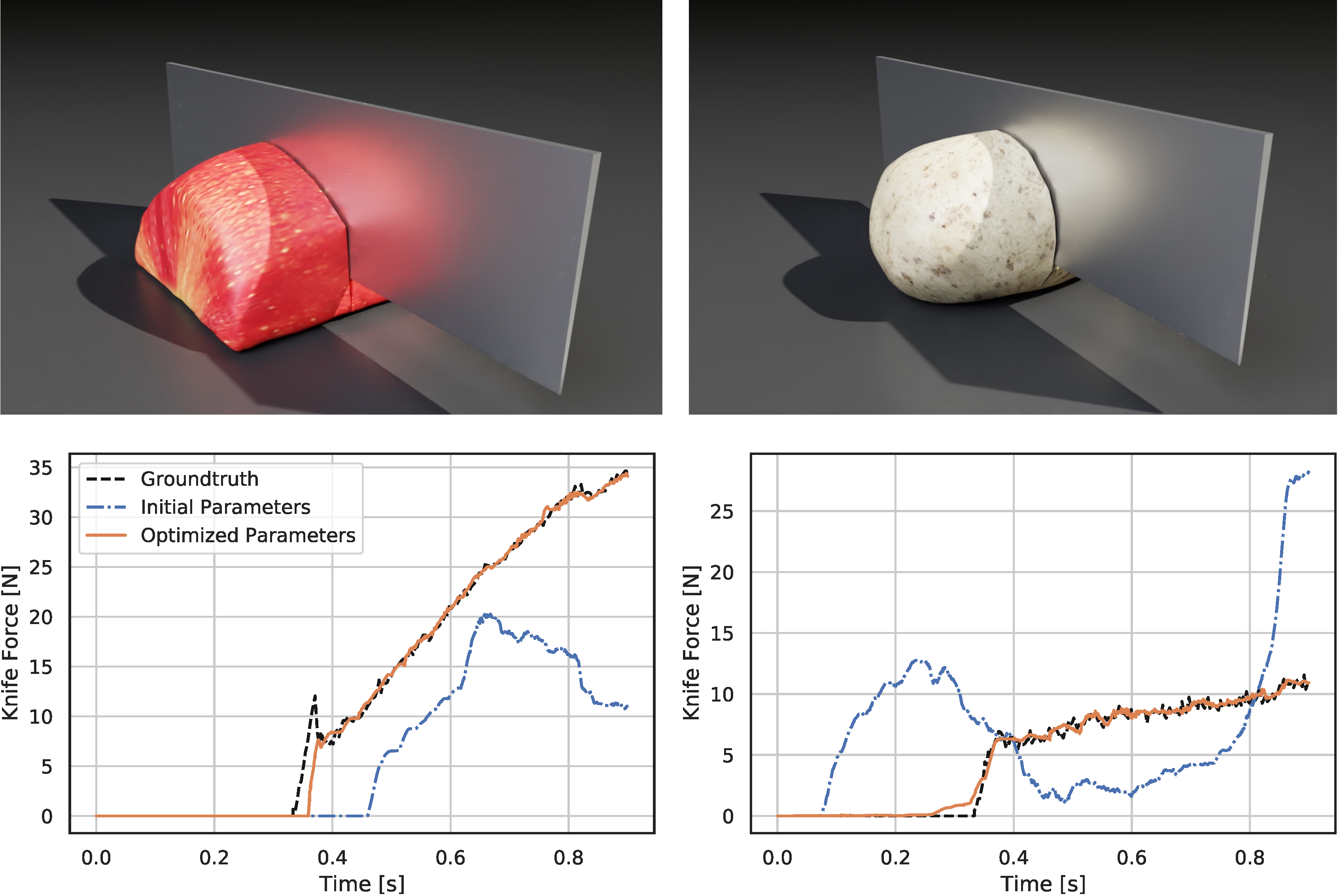
Robotics researchers from NVIDIA and University of Southern California presented their work at the 2021 Robotics: Science and Systems (RSS) conference called DiSECt, the first differentiable simulator for robotic cutting. The simulator accurately predicts the forces acting on a knife as it presses and slices through natural soft materials, such as fruits and vegetables.
Robots that are intelligent, adaptive and generalize cutting behavior with either a kitchen butter knife, or a surgical resection remains a difficult problem for researchers.
As it turns out, the process of cutting with feedback requires adaptation to stiffness of the objects, applied force during the cut, and often a sawing motion to cut through. To achieve this, researchers use a family of techniques which leverage feedback to guide the controller adaptation. However, fluid controller adaptation requires very careful parameter tuning for each instance of the same problem. While these techniques are successful in industrial settings, no two cucumbers (or tomatoes) are the same, hence rendering these family of algorithms ineffective in a more generic setting.
In contrast, recent focus in research has been in building differentiable algorithms for control problems, which in simpler terms means that the sensitivity of output with respect to input can be evaluated without excessive sampling. Efficient solutions for control problems are achievable when the simulated dynamics is differentiable [1,2,3], but the process of simulating cutting has not been differentiable so far!
Differentiable simulation for cutting poses a challenge, since naturally cutting is a discontinuous process where crack formation and fracture propagation occur that prohibit the calculation of gradients. We tackle this problem by proposing a novel way of simulating cutting that represents the process of crack propagation and damage mechanics in a continuous manner.
DiSECt implements the commonly used Finite Element Method (FEM) to simulate deformable materials, such as foodstuffs. The object to be cut is represented by a 3D mesh which consists of tetrahedral elements. Along the cutting surface we slice the mesh following the Virtual Node Algorithm [4]. This algorithm duplicates the mesh elements that intersect the cutting surface, and adds additional, so-called “virtual” vertices on the edges where these elements are cut. The virtual nodes add extra degrees of freedom to accurately simulate the contact dynamics of the knife when it presses and slices through the mesh.
Next, DiSECt inserts springs connecting the virtual nodes on either side of the cutting surface. These cutting springs allow us to simulate damage mechanics and crack propagation in a continuous manner, by weakening them in proportion to the contact force the knife exerts on the mesh. This continuous treatment allows us to differentiate through the dynamics in order to compute gradients for the parameters defining the properties of the material or the trajectory of the knife. For example, given the gradients for the vertical and sideways velocity of the knife, we can efficiently determine an energy-minimizing yet fast cutting motion through gradient-based optimization.
Video: Deformable objects are simulated via the Finite Element Method (FEM). To simulate crack propagation and damage, we insert springs (shown in cyan) between the cut elements of the mesh which are weakened as the knife exerts contact forces.
We leverage reverse-mode automatic differentiation to efficiently compute gradients for hundreds of simulation parameters. Our simulator uses source code transformation which automatically generates efficient CUDA kernels for the forward and backward passes of all our simulation routines, such as the FEM or contact model. Such an approach allows us to implement complex simulation routines which are parallelized on the GPU, while the gradients of the inputs with respect to the outputs of such routines are automatically derived from analyzing the abstract syntax tree (AST) of the simulation code.
Through gradient-based optimization algorithms, we can automatically tune the simulation parameters to achieve a close match between the simulator and real-world measurements. In one of our experiments, we leverage an existing dataset [5] of knife force profiles measured by a real-world robot while cutting various foodstuffs. We set up our simulator with the corresponding mesh and its material properties, and optimize the remaining parameters to reduce the discrepancy between the simulated and the real knife force profile. Within 150 gradient evaluations, our simulator closely predicts the knife force profile, as we demonstrate on the examples of cutting an actual apple and a potato. As shown in the figure, the initial parameter guess yielded a force profile that was far from the real observation, and our approach automatically found an accurate fit. We present further results in our accompanying paper that demonstrate that the found parameters generalize to different conditions, such as the downward velocity of the knife or the length of the reference trajectory window.
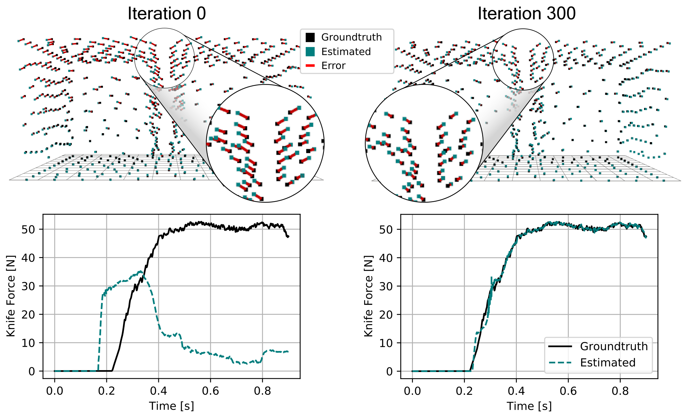
Evolution of the knife force profile while the simulation parameters are calibrated via gradient-based optimization. The ground-truth trajectory has been obtained from a real force sensor attached to a robot cutting a real apple.
We also generate additional data using a highly established commercial simulator, which allows us to precisely control the experimental setup, such as object shape and material properties. Given such data, we can also leverage the motion of the mesh vertices as an additional ground-truth signal. After optimizing the simulation parameters, DiSECt is able to predict the vertex positions and velocities, as well as the force profile, much more accurately.
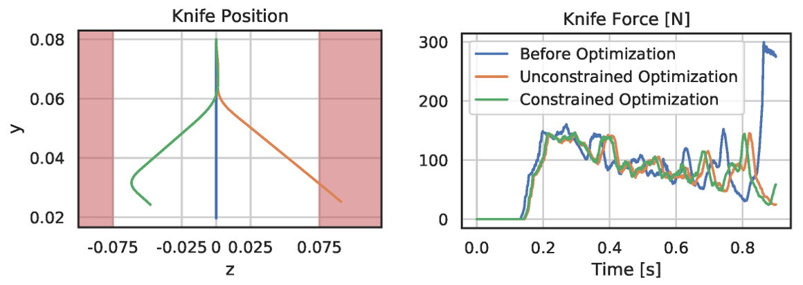
Aside from parameter inference, the gradients of our differentiable cutting simulator can also be used to optimize the cutting motion of the knife. In our full cutting simulation, we represent a trajectory by keyframes, where each frame prescribes the downward velocity, as well as the frequency and amplitude of a sinusoidal sideways velocity. At the start of the optimization, the initial motion is a straight downward-pressing motion.
We optimize this trajectory with the objective to minimize the mean force on the knife and penalize the time it takes to cut the object. Studies have shown that humans perform sawing motions when cutting biomaterials in order to reduce the required force. Such behavior emerges from our optimization as well.
After 50 iterations with the Adam optimizer, we see a reduction in average knife force by 15 percent. However, the knife slices sideways further than its blade length. Therefore, we add a hard constraint to keep the lateral motion within valid limits and perform constrained optimization. Thanks to the end-to-end-differentiability of DiSECt, accurate gradients for such constraints are available, and lead to a valid knife motion which requires only 0.3 percent more force than the unconstrained result.
Cutting food items multiple times results in slightly different force profiles for each instance, depending on the geometry of such materials. We additionally present results to transfer simulation parameters between different meshes corresponding to the same material. Our approach leverages optimal transport to find correspondences between simulation parameters of a source mesh and a target mesh (e.g., local stiffnesses) based on the location of the virtual nodes. As shown in the following figure, the 2D positions of these nodes along the cutting surface allow us to map simulation parameters (shown here is the softness of the cutting springs) to topologically different target geometries.
In our ongoing research, we are bringing our differentiable simulation approach to real-world robotic cutting. We investigate a closed-loop control system where the simulator is updated online from force measurements, while the robot is cutting foodstuffs. Through model-predictive planning and optimal control, we aim to find time- and energy-efficient cutting actions that apply to the physical system.
Hello. I convert weights from a pytorch model to tf2 model. To verify the result, I export the feature maps after the conv2d for both pytorch original model and tf2 model. However, the feature map from tf2 model has black bars on the top and left hand side of the map, whereas the pytorch feature map does not have these black bars.
x = tensorflow.keras.layers.ZeroPadding2D(padding=((2,2)))(inp) x2 = tensorflow.keras.layers.Conv2D(56, 5, padding="valid")(x)
However, the black bar is still there. I have no clue for this problem > <. For the converting process for pytorch weights to tensorflow weights is as follow:

 NVIDIA Optical Flow SDK exposes the APIs to use this Optical Flow hardware (also referred to as NVOFA) to accelerate applications.
 GPU and GPU
 Hosted by the Department of Veterans Affairs (VA), the sprint is designed to foster collaboration with industry and academic partners on AI-enabled tools that leverage federal data to address a need for veterans.
 Targeting areas populated with disease-carrying mosquitoes just got easier thanks to a new study. The research, recently published in IEEE Explore, uses deep learning to recognize tiger mosquitoes from images taken by citizen scientists with near perfect accuracy. “Identifying the mosquitoes is fundamental, as the diseases they transmit continue to be a major public health …


 Developers can use the new viisights wise application powered by GPU-accelerated AI technologies to help organizations and municipalities worldwide avoid operational hazards and risk in their most valuable spaces.
  Robotics researchers from NVIDIA and University of Southern California recently presented their work at the 2021 RSS conference called DiSECt, the first differentiable simulator for robotic cutting.

