Code Reading은 잘 작성되어 있는 프레임워크, 라이브러리, 툴킷 등의 다양한 프로젝트의 내부를 살펴보는 시리즈 입니다. 프로젝트의 아키텍처, 디자인철학이나 코드 스타일 등을 살펴보며, 구체적으로 하나하나 살펴보는 것이 아닌 전반적이면서 간단하게 살펴봅니다.
이번 포스트에서는 프로젝트는 아니지만, 코드 자체와 관련이 깊은 Python 언어의 코드 스타일에 대해서 알아봅니다.
Series.
- CodeReading – 1. PyTorch
- CodeReading – 2. Flask
- CodeReading – 3. ABC
- CodeReading – 4. Python Code Style
Code Style의 중요성
코드스타일이 의미하는 것은 무엇이고, 왜 필요할까요?
코드스타일은 코드 가독성을 위해서 네이밍, 라인수, Indentation 등의 코드의 형식을 맞추는 것을 의미합니다. 이 활동은 특히 ‘협업’에 중점두고 있습니다. 즉 개인이 아닌 팀으로 일하는 경우에 사용하는 하나의 룰 혹은 가이드입니다.
이 Code Reading 시리즈에서 코드를 읽고 있는 것처럼, 코드는 기계 뿐만 아니라 사람들에게도 읽히게 됩니다. 특히 가장 많이 보게 되는 코드는 같이 협업을 하는 동료의 코드일 것 입니다. 이렇게 읽어야 하는 코드가 개인의 코드스타일에 따라서 작성되어 있다면 어떨까요? 스타일에 따라서 다르겠지만, 기본적으로 코드를 해석하는데 시간이 더 걸리게 될 것입니다. 하지만 팀 내부적으로 코드 스타일을 맞춰놓았다면, 훨씬 빠르게 로직을 이해할 수 있고 새롭게 기능을 추가하거나, 코드 리뷰를 하는 등의 다양한 활동을 조금 더 쉽게 진행할 수 있을 것 입니다.
이렇게 명확한 장점을 가지고 있는 코드스타일을 도입하는데 있어서, 한가지 주의할 점이 있습니다. 코드 스타일을 지원하는 다양한 툴이 있기도 하고, 회사마다 스타일 가이드가 있습니다. 즉 누군가에게 조금 더 선호되는 스타일이 있을 수 있지만, 딱 ‘이 스타일이 정답이다’ 라고 말할 수 없는 논술 문제에 가깝습니다. 그래서 팀 내부적으로 의논을 통해, 우리 팀에 맞는 스타일을 모두의 동의하에 정의하고 서로 맞춰나가는 것이 가장 중요합니다.
그렇다면 Pyhon Code Style에 대해서 조금 더 자세히 알아볼까요?

PEP8
Python 언어의 코드 스타일의 가장 기본이 되는 것은 PEP8 입니다. PEP(Python Enhance Proposal)은 공식적으로 운영되고 있는 개선 제안서로서, 그 중에서 PEP8 은 Style Guide for Python Code 이라는 제목으로 작성이 되어있습니다.
여기에는 다음과 같은 가이드들이 작성되어 있습니다. 간략하게 다뤄보면 다음과 같습니다.
- Indentation
# Correct:
# Aligned with opening delimiter.
foo = long_function_name(var_one, var_two,
                         var_three, var_four)

# Add 4 spaces (an extra level of indentation) to distinguish arguments from the rest.
def long_function_name(
        var_one, var_two, var_three,
        var_four):
    print(var_one)

# -------------------------
# Wrong:
# Arguments on first line forbidden when not using vertical alignment.
foo = long_function_name(var_one, var_two,
    var_three, var_four)

# Further indentation required as indentation is not distinguishable.
def long_function_name(
    var_one, var_two, var_three,
    var_four):
    print(var_one)
indentation의 경우, 함수의 arguments 들이 명확히 구별되도록 가이드하고 있습니다.
- Tabs vs Spaces
PEP8에서는 Space를 써야한다고 이야기하고 있고, 두가지를 혼합해서 사용하는 것을 금지하고 있습니다! (이 포스트 시작에 있는 그림과 연결되죠)
- 권장사항
아래와 같이 empty sequence 는 False 인 것을 이용해서, length를 기반으로 체크하지 않도록 권장하기도 합니다.
# Correct:
if not seq:
if seq:

# Wrong:
if len(seq):
if not len(seq):
가장 기본이 되는 스타일 가이드이기 때문에 전체를 한번 읽어보실 것을 추천드립니다. 대부분의 내용은 지금도 사용되고 있습니다. 다만, PEP8이 제안될 당시와 비교했을 때 개발 환경은 많이 달라졌습니다. 작은 모니터에서 다양한 크기의 모니터를 여러개 연결해서 개발을 하는 것이 흔해진 상황이죠. 그래서 Maximum Line Length의 경우에는 의견이 분분하기도 합니다. 모든 행을 79자 제한으로 제안되었지만, 더 길게 셋팅을 하는 경우도 흔하게 찾아볼 수 있습니다.
Tools
코드스타일에 관련한 도구들은 위의 PEP8을 기본으로 지원하면서 환경셋팅을 통해서 원하는대로 수정할 수 있도록 되어있습니다. 여러가지 도구들이 있지만, 최근에 가장 많이 사용하고 있는 black과 isort 두가지를 대표적으로 소개해드려고 합니다.
black
The Uncompromising Code Formatter
black은 비교적 최근(2018년)에 개발된 오픈소스로 정해진 코드의 규격에 맞춰서 정리해주는 Code Formatter 입니다. black의 가장 큰 특징은 바로 ‘타협하지 않는’ 입니다. 타협하지 않는 부분은 바로 PEP8 에서 커버하지 않고 있는, 사람마다 각각 스타일이 다른 부분입니다. 그래서 black의 공식 문서에서도 PEP을 준수하는 엄격한 하위집단이라고 이야기 하고 있습니다.
그러면 black에서 추구하는 코드 스타일에 대해서 간단하게 살펴보겠습니다.
- Maximum Line Length : 88 (80 에서 10% 늘어난 값)
- 줄 바꿈 방식
# [1] in:
ImportantClass.important_method(exc, limit, lookup_lines, capture_locals, extra_argument)

# [1] out:
ImportantClass.important_method(
    exc, limit, lookup_lines, capture_locals, extra_argument
)

# [2] in:
def very_important_function(template: str, *variables, file: os.PathLike, engine: str, header: bool = True, debug: bool = False):
    """Applies `variables` to the `template` and writes to `file`."""
    with open(file, 'w') as f:
        ...

# [2] out:
def very_important_function(
    template: str,
    *variables,
    file: os.PathLike,
    engine: str,
    header: bool = True,
    debug: bool = False,
):
    """Applies `variables` to the `template` and writes to `file`."""
    with open(file, "w") as f:
        ...

# [3] in:
if some_long_rule1
  and some_long_rule2:
    ...

# [3] out:
if (
    some_long_rule1
    and some_long_rule2
):
    ...
줄 길이에 따라서 위와 같이, 들여쓰기[1]가 되거나 파라미터가 더욱 많은 경우에는 하나하나 새로운 줄[2]에 위치하게 됩니다. 그리고 문장 길이를 맞추기 위해서 사용하는 백슬래시()가 파싱오류 등의 이슈가 있기 때문에 이를 사용하지 않는다고 말하고 있습니다.
- String: 작은따옴표(‘) 보다는 큰따옴표(“)를 선호
doc string에서도 큰따옴표(“)를 사용하고 있고, 큰따옴표로 구성된 empty string의 경우 (“”) 혼동을 줄 여지가 없기 때문이죠.
- Call chains
def example(session):
    result = (
        session.query(models.Customer.id)
        .filter(
            models.Customer.account_id == account_id,
            models.Customer.email == email_address,
        )
        .order_by(models.Customer.id.asc())
        .all()
    )
마지막으로 많은 언어에서 사용되고 있는 call chain 형식 또한 사용하고 있습니다. 저는 개인적으로 Java 와 Scala에서 이런 패턴을 많이 봐서 더 익숙하기도 하고, 어떤 로직인지 이해가기가 쉬워서 선호하는 스타일이기도 합니다.
그 외에도 다양한 주제들이 있으니 문서를 참고해보시기를 추천드립니다!
black 에서 추구하고 있는 코드스타일이 모호한 부분들을 다루고 있는 것처럼, 모두가 여기서 제안하는 스타일이 만족스럽지 않을 수 있습니다. 협업을 위한 코드스타일에 좋은 가이드이자 시작점이 아닐까 싶습니다.
isort
isort는 import 를 관리해주는 Code Formatter 입니다. 아래 예시를 보시면 바로 감이 잡히실 것 같네요.
# Before isort:
from my_lib import Object

import os

from my_lib import Object3

from my_lib import Object2

import sys

from third_party import lib15, lib1, lib2, lib3, lib4, lib5, lib6, lib7, lib8, lib9, lib10, lib11, lib12, lib13, lib14

import sys

from __future__ import absolute_import

from third_party import lib3

print("Hey")
print("yo")

# ----------------------------------------------------------------------
# After isort:
from __future__ import absolute_import

import os
import sys

from third_party import (lib1, lib2, lib3, lib4, lib5, lib6, lib7, lib8,
                         lib9, lib10, lib11, lib12, lib13, lib14, lib15)

from my_lib import Object, Object2, Object3

print("Hey")
print("yo")
위의 예제에서 보는 것처럼, import 되는 package의 종류를 아래 4가지로 관리하고 있습니다.
__future__: Python2 에서 3의 기능을 사용하기 위해서 Import 하는 모듈built-in modules: os, sys, collections 등 Python의 기본 내장 모듈third party: pip를 통해서 설치한 외부 library 들 (e.g. requests, pytorch 등)my library: 스스로 만든 package
black 과의 큰 차이점은 다양한 옵션들을 제공하는 것입니다. 위의 예시에서 third_party 의 모듈 여러개를 import 하는 방식에서 한 줄로 나열하는 방식, 하나씩 줄을 바꾸는 경우 등 다양한 옵션들이 있는 것을 확인하실 수 있습니다.
# 0 - Grid
from third_party import (lib1, lib2, lib3,
                         lib4, lib5, ...)

# 1 - Vertical
from third_party import (lib1,
                         lib2,
                         lib3
                         lib4,
                         lib5,
                         ...)

...
# 3 - Vertical Hanging Indent (Black Style)
from third_party import (
    lib1,
    lib2,
    lib3,
    lib4,
)

...
관련해서 옵션이 11개 있으니, 원하는 대로 설정해서 사용하시면 될 것 같습니다. 만약에 위에서 소개했던 black과 같이 사용한다면 3번 옵션으로 셋팅해서 사용하면 스타일을 유지할 수 있게 됩니다. isort 에서는 다른 Code Formatter 라이브러리들끼리는 서로가 호환되도록 개발을 모두 해놓았기 때문에 간단한 설정으로 양쪽 모두 사용하실 수 있을 것 입니다.
끝으로
이번 포스트에서는 Code Style을 왜 맞추어야 하는지 그리고 Python 코드 스타일 가이드 PEP8에서 시작해서 쉽게 적용해볼 수 있는 Tool 을 소개시켜 드렸습니다. 서문에서 이야기 한 것처럼, 코드 스타일은 다른 무엇이 아닌 협업을 위한 것 입니다. 그래서 코드 스타일 자체보다는 이것을 도입하기 까지의 과정이 더 중요하다고 생각이 드네요. ‘함께’ 더 잘 일하기 위한 것이니까요.
 Simulated or synthetic data generation is an important emerging trend in the development of AI tools. Classically, these datasets can be used to address low-data problems or edge-case scenarios that might now be present in available real-world datasets. Emerging applications for synthetic data include establishing model performance levels, quantifying the domain of applicability, and next-generation …
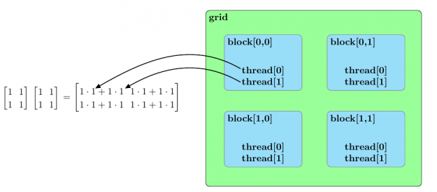
![[A cdot B]](https://s0.wp.com/latex.php?latex=%5BA+%5Ccdot+B%5D&bg=ffffff&fg=000&s=0&c=20201002) to be well defined, the number of columns of
to be well defined, the number of columns of ![[A]](https://s0.wp.com/latex.php?latex=%5BA%5D&bg=ffffff&fg=000&s=0&c=20201002) must be equal to the number of rows of
must be equal to the number of rows of ![[B]](https://s0.wp.com/latex.php?latex=%5BB%5D&bg=ffffff&fg=000&s=0&c=20201002) .
.![[m]](https://s0.wp.com/latex.php?latex=%5Bm%5D&bg=ffffff&fg=000&s=0&c=20201002) rows and
rows and ![[n]](https://s0.wp.com/latex.php?latex=%5Bn%5D&bg=ffffff&fg=000&s=0&c=20201002) columns, that is, an
columns, that is, an ![[m times n]](https://s0.wp.com/latex.php?latex=%5Bm+%5Ctimes+n%5D&bg=ffffff&fg=000&s=0&c=20201002) matrix.
matrix.![[n times p]](https://s0.wp.com/latex.php?latex=%5Bn+%5Ctimes+p%5D&bg=ffffff&fg=000&s=0&c=20201002) matrix.
matrix.![[C = A cdot B]](https://s0.wp.com/latex.php?latex=%5BC+%3D+A+%5Ccdot+B%5D&bg=ffffff&fg=000&s=0&c=20201002) results in an
results in an ![[m times p]](https://s0.wp.com/latex.php?latex=%5Bm+%5Ctimes+p%5D&bg=ffffff&fg=000&s=0&c=20201002) matrix.
matrix.![[C]](https://s0.wp.com/latex.php?latex=%5BC%5D&bg=ffffff&fg=000&s=0&c=20201002) ,
, ![[C[i,j]]](https://s0.wp.com/latex.php?latex=%5BC%5Bi%2Cj%5D%5D&bg=ffffff&fg=000&s=0&c=20201002) , is determined by the following formula:
, is determined by the following formula:![[C[i,j] = Sigma_{r = 1}^{n} A[i,r] cdot B[r,j]]](https://s0.wp.com/latex.php?latex=%5BC%5Bi%2Cj%5D+%3D+%5CSigma_%7Br+%3D+1%7D%5E%7Bn%7D+A%5Bi%2Cr%5D+%5Ccdot+B%5Br%2Cj%5D%5D&bg=ffffff&fg=000&s=0&c=20201002)
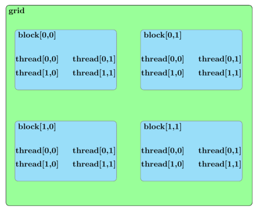
![[textrm{nblocksx}]](https://s0.wp.com/latex.php?latex=%5B%5Ctextrm%7Bnblocksx%7D%5D&bg=ffffff&fg=000&s=0&c=20201002) ) is greater than or equal to
) is greater than or equal to ![[textrm{nblocksx} geq m]](https://s0.wp.com/latex.php?latex=%5B%5Ctextrm%7Bnblocksx%7D+%5Cgeq+m%5D&bg=ffffff&fg=000&s=0&c=20201002) ).
).![[textrm{nblocksy}]](https://s0.wp.com/latex.php?latex=%5B%5Ctextrm%7Bnblocksy%7D%5D&bg=ffffff&fg=000&s=0&c=20201002) ) is greater than or equal to
) is greater than or equal to ![[p]](https://s0.wp.com/latex.php?latex=%5Bp%5D&bg=ffffff&fg=000&s=0&c=20201002) (
(![[textrm{nblocksy} geq p]](https://s0.wp.com/latex.php?latex=%5B%5Ctextrm%7Bnblocksy%7D+%5Cgeq+p%5D&bg=ffffff&fg=000&s=0&c=20201002) ).,
).,![[textrm{nthreads}]](https://s0.wp.com/latex.php?latex=%5B%5Ctextrm%7Bnthreads%7D%5D&bg=ffffff&fg=000&s=0&c=20201002) ) is greater than or equal to
) is greater than or equal to ![[textrm{nthreads} geq n]](https://s0.wp.com/latex.php?latex=%5B%5Ctextrm%7Bnthreads%7D+%5Cgeq+n%5D&bg=ffffff&fg=000&s=0&c=20201002) ).
).![[textrm{tid}(i,j)]](https://s0.wp.com/latex.php?latex=%5B%5Ctextrm%7Btid%7D%28i%2Cj%29%5D&bg=ffffff&fg=000&s=0&c=20201002) denoting the thread index of a thread belonging to a block with indices in the grid of
denoting the thread index of a thread belonging to a block with indices in the grid of ![[[i,j]]](https://s0.wp.com/latex.php?latex=%5B%5Bi%2Cj%5D%5D&bg=ffffff&fg=000&s=0&c=20201002) . The preceding parallel arrangement can be summarized by the following equation:
. The preceding parallel arrangement can be summarized by the following equation:![[C[i,j] = textrm{atomicAdd}(C[i,j], A[i, textrm{tid}(i,j)] cdot B[textrm{tid}(i,j), j])]](https://s0.wp.com/latex.php?latex=%5BC%5Bi%2Cj%5D+%3D+%5Ctextrm%7BatomicAdd%7D%28C%5Bi%2Cj%5D%2C+A%5Bi%2C+%5Ctextrm%7Btid%7D%28i%2Cj%29%5D+%5Ccdot+B%5B%5Ctextrm%7Btid%7D%28i%2Cj%29%2C+j%5D%29%5D&bg=ffffff&fg=000&s=0&c=20201002)
![[2 times 2]](https://s0.wp.com/latex.php?latex=%5B2+%5Ctimes+2%5D&bg=ffffff&fg=000&s=0&c=20201002) .
.
![[N times N]](https://s0.wp.com/latex.php?latex=%5BN+%5Ctimes+N%5D&bg=ffffff&fg=000&s=0&c=20201002) matrices with all elements of both matrices equal to one.
matrices with all elements of both matrices equal to one. ![[N]](https://s0.wp.com/latex.php?latex=%5BN%5D&bg=ffffff&fg=000&s=0&c=20201002) ranges from one hundred to one thousand in increments of one hundred.
ranges from one hundred to one thousand in increments of one hundred.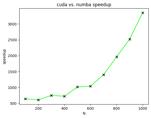
![[mathcal{O}(N^{2})]](https://s0.wp.com/latex.php?latex=%5B%5Cmathcal%7BO%7D%28N%5E%7B2%7D%29%5D&bg=ffffff&fg=000&s=0&c=20201002) problem when implemented as a direct calculation. Fortunately, NVIDIA has developed a ray tracing library, named NVIDIA OptiX, which uses GPU parallelism to achieve significant speedups. Use of NVIDIA OptiX from within a Blender Python environment would then offer tangible benefits.
problem when implemented as a direct calculation. Fortunately, NVIDIA has developed a ray tracing library, named NVIDIA OptiX, which uses GPU parallelism to achieve significant speedups. Use of NVIDIA OptiX from within a Blender Python environment would then offer tangible benefits. Learn about the latest GPU Operator releases which include support for multi-instance GPU Support, pre-installed NVIDIA drivers, Red Hat OpenShift 4.7, and more.
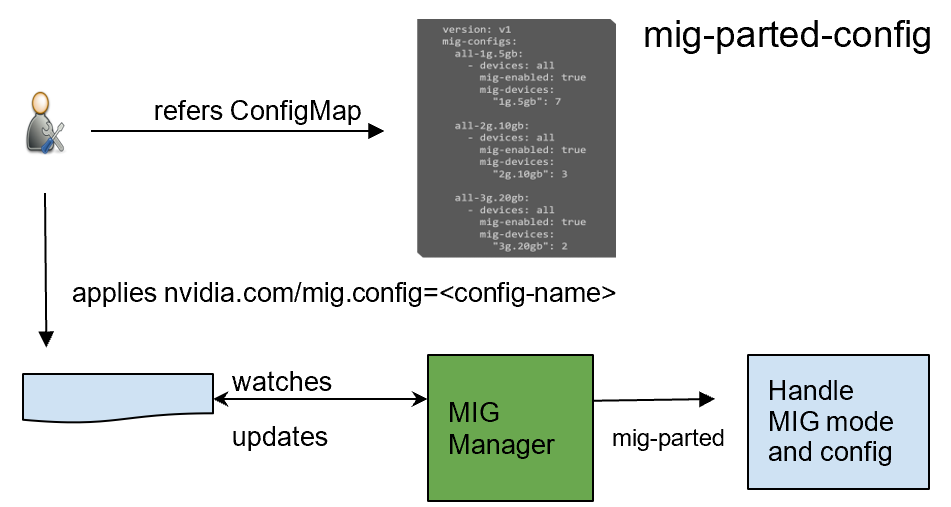
 Is EVPN magic? As Arthur C Clarke said, any sufficiently advanced technology is indistinguishable from magic. On that premise, moving from a traditional layer 2 environment to VXLAN driven by EVPN has much of that same hocus-pocus feeling. To help demystify the sorcery, I aim to help users new to EVPN understand how EVPN works …
  This posts compares asymmetric and symmetric EVPN routing models using EVPN as the control plane. It provides architecture differences and maps them to specific NOS CLI output for educational purposes.
 Industry luminaries joined us to introduce the fundamentals of real-time ray tracing, and how current developers such as Autodesk, Dassault, Chaos and ESI have integrated ray traced technologies into their most popular apps.
 The NVIDIA NGC catalog is a hub of highly performant software containers, pre-trained models, industry specific SDKs and Helm charts you can simplify and accelerate your end-to-end workflows.
  The Game Developer Conference (GDC) is here, and NVIDIA will be showcasing how our latest technologies are driving the future of game development and graphics. Check out our list of sessions now.